Fit Sigmoidal Models

Sigmoidal models are S-shaped curves that are commonly used to model dose-response curves and population dynamics. These models are also used in many artificial neural networks as activation functions. Curve Fitting Toolbox™ supports logistic, 4-parameter logistic, and Gompertz sigmoidal models with the following equations.

Sigmoidal Model	Equation
Logistic	$$f(x)=\frac{a}{1+e^{-b(x-c)}}$$
4-parameter logistic	$$f(x)=d+\frac{a-d}{1+{\left(\frac{x}{c}\right)}^b}$$
Gompertz	$$f(x)=d+(a-d)e^{-e^{-b(x-c)}}$$

In these equations, a and d are parameters for the horizontal asymptotes, and b is a growth rate parameter. For a 4-parameter logistic model, the input data x must contain all positive or all negative elements, and c is the midpoint between the horizontal asymptotes. For a Gompertz model, c is the inflection point for the curve. For a logistic model, c is both the midpoint and the inflection point.

Fit Sigmoidal Model Using Curve Fitter App

Generate data with added noise by using the linspace, exp, and randn functions, and the standard logistic function $$p(x)=\frac{1}{1+e^{-x}}$$. p, which is bounded between 0 and 1, represents the probability of an event occurring given the input x.

rng(0,"twister") %  For reproducibility
x = linspace(-5,5,100)';
p = 1./(1+exp(-x)) + 0.02*randn(100,1);
p(p>1) = 1;
p(p<0) = 0;

Open the Curve Fitter app from the command line.

curveFitter

Alternatively, on the Apps tab, in the Math, Statistics, and Optimization group of the apps gallery, click Curve Fitter.

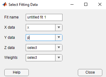
In the app, select the data variables for the fit. On the Curve Fitter tab, in the Data section, click Select Data. In the Select Fitting Data dialog box, select x as the X data value and p as the Y data value.

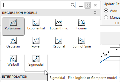
The app plots the data points as you select variables. By default, the app fits a linear polynomial to the data. To fit a sigmoidal model, click Sigmoidal in the Fit Type gallery of the Curve Fitter tab.

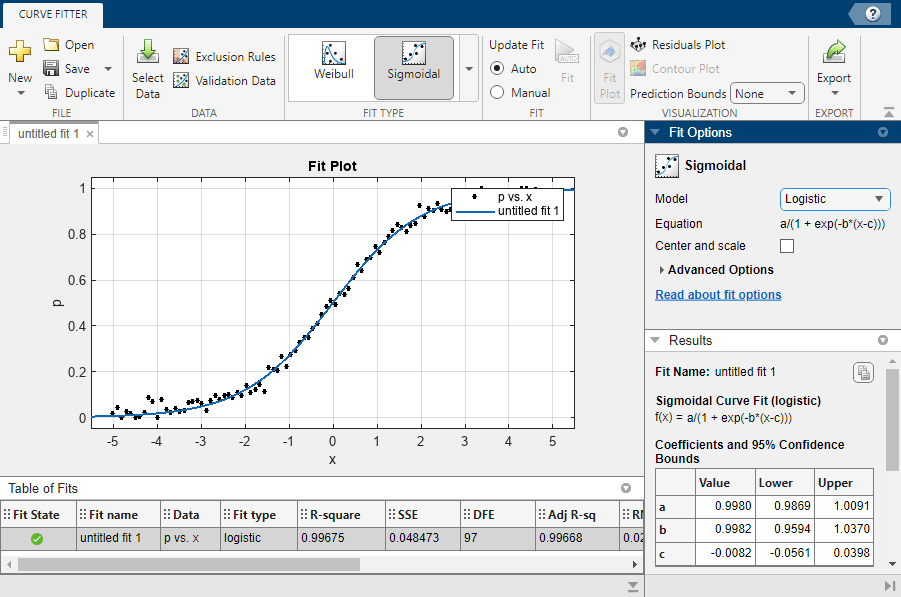
By default, the app plots a logistic model.

The plot shows that the logistic fit follows the bulk of the data. The probability is small for negative values of x, then increases, and then plateaus around 1. The Table of Fits shows the goodness-of-fit statistics for the logistic model, including the sum of squares error (SSE) of approximately 0.048, and the R-square value of approximately 1. The Results pane also displays the model equation and the fitted coefficients with 95% confidence bounds.

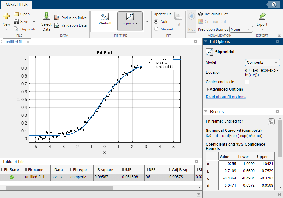
To use a different model equation, select a different model name from the Model menu in the Fit Options pane. For example, you can select a Gompertz model.

The plot shows that the lower asymptote for the Gompertz curve is greater than zero. The Table of Fits shows that this fit has a larger SSE value and a slightly smaller R-square value compared to the logistic fit. This result is due to the data being generated from a Gompertz function rather than a logistic function.

Fit Sigmoidal Model at Command Line

Generate data with added noise by using the linspace, tanh, and randn functions.

rng(0,"twister") %  For reproducibility
pts = linspace(-5,5,100)';
x = linspace(1,11,100)';
y = tanh(pts)+0.1*randn(100,1);

The vector x contains data for the independent variable, and the vector y contains data for the dependent variable.

Use the scatter function to create a scatter plot of the data in x and y.

scatter(x,y)

The scatter plot shows that y contains positive and negative values, x contains all positive values, and the data follows an S-shape.

Fit a 4-parameter logistic model to x and y.

f = fit(x,y,'logistic4')

f = 
     General model Logistic4:
     f(x) = d + (a-d)/(1 + (x/c)^b)
     Coefficients (with 95% confidence bounds):
       a =     -0.9507  (-0.989, -0.9125)
       b =       12.93  (11.14, 14.72)
       c =       6.013  (5.94, 6.086)
       d =       1.003  (0.9608, 1.046)

f is a cfit object that contains the results of fitting a 4-parameter logistic model to the data.

Plot f together with x and y.

plot(f,x,y)

The plot shows that the fitted curve f follows the bulk of the data.

References

[1] Tjørve, Kathleen M. C., and Even Tjørve. “The Use of Gompertz Models in Growth Analyses, and New Gompertz-Model Approach: An Addition to the Unified-Richards Family.” PLOS ONE, edited by Roeland M.H. Merks, vol. 12, no. 6, June 2017, p. e0178691. DOI.org (Crossref), https://doi.org/10.1371/journal.pone.0178691.