Approximate Different Delays with Different Approximation Orders
This example shows how to specify different Padé approximation orders to approximate internal and output delays in a continuous-time open-loop system.
Load a sample continuous-time open-loop system that contains internal and output time delays.
load('PadeApproximation1.mat','sys')
sys
sys =

  A =
         x1    x2
   x1  -1.5  -0.1
   x2     1     0

  B =
       u1
   x1   1
   x2   0

  C =
        x1   x2
   y1  0.5  0.1

  D =
       u1
   y1   0

  (values computed with all internal delays set to zero)

  Output delays (seconds): 1.5
  Internal delays (seconds): 3.4

Continuous-time state-space model.
Model Properties
sys is a second-order continuous-time ss model with internal delay 3.4 s and output delay 1.5 s.
Use the pade function to compute a third-order approximation of the internal delay and a first-order approximation of the output delay.
P13 = pade(sys,inf,1,3);
size(P13)
State-space model with 1 outputs, 1 inputs, and 6 states.
The three input arguments following sys specify the approximation orders of any input, output, and internal delays of sys, respectively. inf specifies that a delay is not to be approximated. The approximation orders for the output and internal delays are one and three respectively.
Approximating the time delays with pade absorbs delays into the dynamics, adding as many states to the model as orders in the approximation. Thus, P13 is a sixth-order model with no delays.
For comparison, approximate only the internal delay of sys, leaving the output delay intact.
P3 = pade(sys,inf,inf,3);
size(P3)
State-space model with 1 outputs, 1 inputs, and 5 states.
P3.OutputDelay
ans =
1.5000
P3.InternalDelay
ans =

  0×1 empty double column vector
P3 retains the output delay, but the internal delay is approximated and absorbed into the state-space matrices, resulting in a fifth-order model without internal delays.
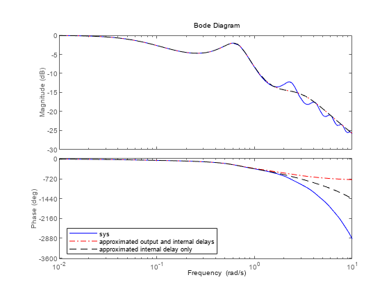
Compare the frequency response of the exact and approximated systems sys, P13, P3.
h = bodeoptions;
h.PhaseMatching = 'on';
bode(sys,'b-',P13,'r-.',P3,'k--',h,{.01,10});
legend('sys','approximated output and internal delays','approximated internal delay only',...
    'location','SouthWest')

Notice that approximating the internal delay loses the gain ripple displayed in the exact system.