Receiver Thermal Noise

Apply receiver thermal noise to complex signal

Libraries:
Communications Toolbox / RF Impairments and Components

Description

The Receiver Thermal Noise block applies receiver thermal noise to a complex signal. The block simulates the effects of thermal noise on a complex signal. The Specification method parameter enables specification of the thermal noise based on the noise temperature, noise figure, or noise factor.

Examples

expand all

Apply Receiver Thermal Noise to QAM Modulated Signal

This example uses:

Open Model

The cm_receiver_thermal_noise_qam model applies receiver thermal noise to a 16-QAM signal, and displays the signal in a constellation diagram. The model applies receiver thermal noise by specifying the noise figure in the Receiver Thermal Noise block.

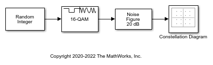
Run the simulation at a sample rate of 1 kHz by setting the sample time to 1e-3 samples per second in the Random Integer Generator block. The Rectangular QAM Modulator Baseband block has the normalization method set to average power and the average power level set to 3e-13 watts (-92.5 dBm). Set the noise figure level in the Receiver Thermal Noise block to 20 dB, and display the constellation diagram of the 16-QAM signal.

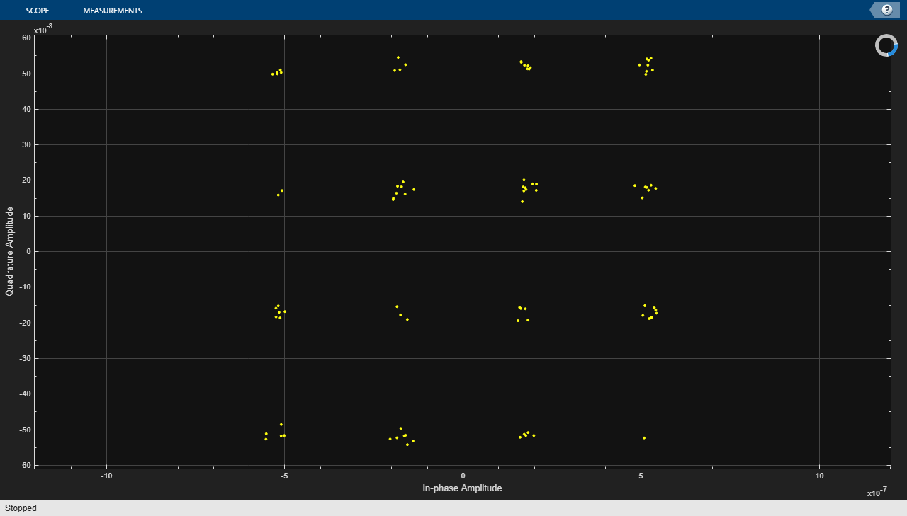
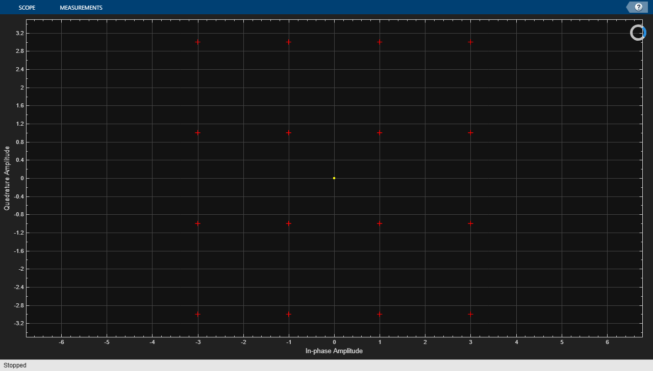
Decreasing the noise figure will reduce the simulated receive noise level, and result in a tighter clustering of samples for the individual points in the constellation diagram. To demonstrate this, set the noise figure level to 10 dB and show the constellation diagram of the 16-QAM signal.

Add RF Impairments to DQPSK Signal

This example uses:

Open Script

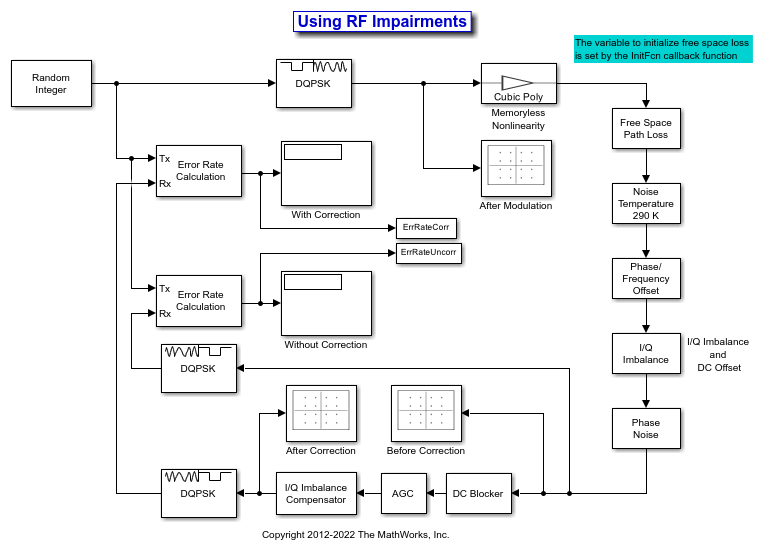
This example applies RF impairments to a signal modulated by the differential quadrature phase shift keying (DQPSK) method. To show the RF impairments, the example applies exaggerated levels that are not typical levels for modern radios.

In this example, the slex_rcvrimpairments_dqpsk model DQPSK-modulates a random signal and applies various RF impairments to the signal. The model uses impairment blocks from the RF Impairments library. The InitFun callback function initializes simulation variables. For more information, see Model Callbacks (Simulink).

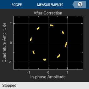
After the impairment blocks, the signal forks into two paths. One path applies DC blocking, automatic gain control (AGC), and I/Q imbalance compensation to the signal before demodulation. The signal on the correction path is adjusted by the DC Blocker, AGC, and I/Q Imbalance Compensator blocks. Because the signal is DQPSK modulated, no carrier synchronization is required. The second path goes directly to demodulation. After demodulation, an error rate calculation is performed on both signals. The model includes Constellation Diagram blocks after modulation, before correction, and after correction so that you can analyze the constellation.

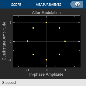
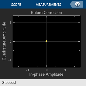
When the model runs, constellation diagrams plot the signal at these stages in the simulation:

The After Modulation constellation diagram shows the reference DQPSK-modulated signal constellation.
The Before Correction constellation diagram shows the attenuated and distorted signal constellation.
The After Correction constellation diagram shows the signal has been amplified and improved after the correction blocks.

The error rate for the demodulated signal without AGC is primarily caused by free space path loss and I/Q imbalance. The QPSK modulation minimizes the effects of the other impairments.

Error rate for corrected signal:   0.000
Error rate for uncorrected signal: 0.042

To explore the model try:

Adjusting RF impairment settings, rerun the model, and notice the changes to the constellation diagrams and error rates.
Modifying the model to add an equalizer stage before the demodulation. Equalization has inherent ability to reduce some of the distortion caused by impairments. For more information, see Equalization.

Extended Examples

RF Satellite Link

Simulate a satellite link that models amplifier impairments by using a Memoryless Nonlinearity block.

Open Script

Ports

Input

expand all

In1 — Complex signal
scalar | column vector

Complex signal, specified as a scalar or column vector.

Data Types: double | single
Complex Number Support: Yes

Output

expand all

Out1 — Output signal
scalar | column vector

Output signal, returned as a scalar or column vector. This output is the same dimension and data type as the input signal.

Parameters

expand all

To edit block parameters interactively, use the Property Inspector. From the Simulink^® Toolstrip, on the Simulation tab, in the Prepare gallery, select Property Inspector.

Specification method — Thermal noise specification method
`Noise temperature` (default) | `Noise figure` | `Noise factor`

Thermal noise specification method, specified as one of these options.

Noise temperature specifies the noise in kelvins.
Noise figure specifies the added receiver noise in dB relative to an input noise temperature of 290 K. The noise figure is the decibel equivalent of the noise factor.
Noise factor specifies the added receiver noise relative to an input noise temperature of 290 K. The noise factor is the linear equivalent of the noise figure.

Noise temperature (K) — Noise temperature
`290` (default) | scalar

Noise temperature in kelvins, specified as a scalar.

Tunable: Yes

Dependencies

To enable this parameter, set the Specification method parameter to Noise temperature.

Noise figure (dB) — Receiver noise figure
`3.0103` (default) | scalar

Receiver noise figure in dB relative to a noise temperature of 290 K, specified as a scalar.

Note

This parameter specifies the noise contribution of the receiver circuitry only. To add the effects of antenna noise, select the Add 290K antenna noise parameter.

Tunable: Yes

Dependencies

To enable this parameter, set the Specification method parameter to Noise figure.

Noise factor — Receiver noise factor
`2` (default) | scalar

Receiver noise factor relative to a noise temperature of 290 K, specified as a scalar.

Note

This parameter specifies the noise contribution of the receiver circuitry only. To add the effects of antenna noise, select the Add 290K antenna noise parameter.

Tunable: Yes

Dependencies

To enable this parameter, set the Specification method parameter to Noise factor.

Add 290K antenna noise — Option to add 290 K antenna noise
`off` (default) | `on`

Select this parameter to add 290 K antenna noise to the signal.

Dependencies

To enable this parameter, set the Specification method parameter to Noise factor or Noise figure.

Reference load (ohm) — Reference load
`1` (default) | scalar

Reference load value in ohms, specified as a scalar. This value is used to compute the voltage levels based on the signal and noise power levels.

Tunable: Yes

Initial seed — Initial seed value
`67987` (default) | scalar

Initial seed value for the random number generator, specified as a scalar.

Block Characteristics

Data Types	`double` \| `single`
Multidimensional Signals	`no`
Variable-Size Signals	`no`

Algorithms

Wireless receiver performance is often expressed as a noise factor or figure. The noise factor is defined as the ratio of the input signal-to-noise ratio, S_i/N_i to the output signal-to-noise ratio, S_o/N_o, such that

$F = \frac{S_{i} / N_{i}}{S_{o} / N_{o}} .$

Given the receiver gain G and receiver noise power N_ckt, the noise factor can be expressed as

$\begin{matrix} F = \frac{S_{i} / N_{i}}{G S_{i} / (N_{c k t} + G N_{i})} \\ = \frac{N_{c k t} + G N_{i}}{G N_{i}} . \end{matrix}$

The IEEE defines the noise factor assuming that noise temperature at the input is T₀, where T₀ = 290 K. The noise factor is then

$\begin{matrix} F = \frac{N_{c k t} + G N_{i}}{G N_{i}} \\ = \frac{G k B T_{c k t} + G k B T_{0}}{G k B T_{0}} \\ = \frac{T_{c k t} + T_{0}}{T_{0}} . \end{matrix}$

T_ckt is the equivalent input noise temperature of the receiver and is expressed as

$T_{c k t} = T_{0} (F - 1) .$

The overall noise temperature of an antenna and receiver T_sys is

$T_{s y s} = T_{a n t} + T_{c k t},$

where T_ant is the antenna noise temperature.

The noise figure NF is the dB equivalent of the noise factor and can be expressed as

$N F = 10 \log_{10} (F) .$

The noise power can be expressed as

$N = k T B = V^{2} / R,$

where V is the noise voltage expressed as

$V^{2} = k T B R,$

and R is the reference load.

Extended Capabilities

C/C++ Code Generation
Generate C and C++ code using Simulink® Coder™.

Version History

Introduced before R2006a

Receiver Thermal Noise

Description

Examples