Port Analysis of Antenna
This example quantifies terminal antenna parameters, with regard to the antenna port. The antenna is a one-port network. The antenna port is a physical location on the antenna where an RF source is connected to it. The terminal port parameters supported in Antenna Toolbox™ are
Antenna impedance
Return loss
S-parameters
VSWR
The example uses a Planar Inverted-F Antenna (PIFA), performs the corresponding computational analysis, and returns all terminal antenna parameters listed above.
Create Inverted-F Antenna
Create the default geometry for the PIFA antenna. The (small) red dot on the antenna structure is the feed point location where an input voltage generator is applied. It is the port of the antenna. In Antenna Toolbox™, all antennas are excited by a time-harmonic voltage signal with the amplitude of 1 V at the port. The port must connect two distinct conductors; it has an infinitesimally small width.
ant = invertedF;
figure
show(ant)
title("Inverted-F Antenna");
Impedance
To plot the antenna impedance, specify the frequency band over which the data needs to be plotted using impedance function. The antenna impedance is calculated as the ratio of the phasor voltage (which is simply 1) and the phasor current at the port.
freq = linspace(1.5e9,2.0e9,51);
figure
impedance(ant,freq);
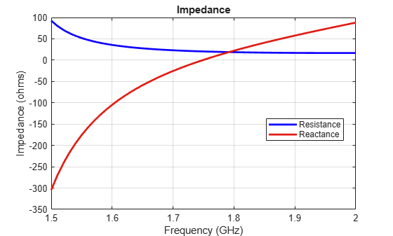
The plot displays the real part of the impedance, i.e. resistance as well as its imaginary part, i.e. reactance, over the entire frequency band. Antenna resonant frequency is defined as the frequency at which the reactance of the antenna is exactly zero. Looking at the impedance plot, we observe that the inverted-F antenna resonates at 1.74 GHz. The resistance value at that frequency is about 20 . The reactance values for the antenna are negative (capacitive) before resonance and become positive (inductive) after resonance, indicating that it is the series resonance of the antenna (modeled by a series RLC circuit). If the impedance curve goes from positive reactance to negative, it is the parallel resonance [1] (modeled by a parallel RLC circuit).
Return Loss
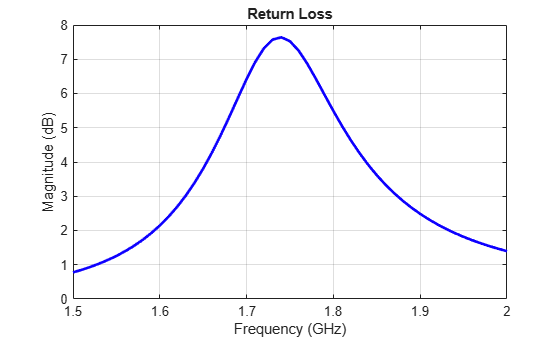
To plot the return loss of an antenna, specify the frequency band over which the data needs to be plotted. Return loss is the measure of the effectiveness of power delivery from the transmission line to an antenna. Quantitatively, the return loss is the ratio, in dB, of the power sent towards the antenna and the power reflected back. It is a positive quantity for passive devices. A negative return loss is possible with active devices [2].
figure
returnLoss(ant,freq);
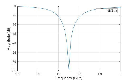
Reflection Coefficient
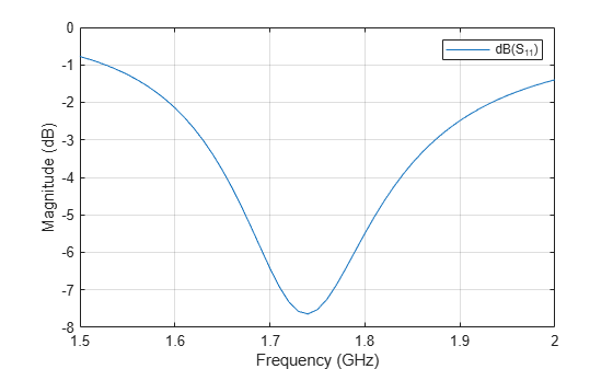
The return loss introduced above is rarely used for the antenna analysis. Instead, a reflection coefficient or in dB is employed, which is also often mistakenly called the "return loss" [2]. In fact, the reflection coefficient in dB is the negative of the return loss as seen in the following figure. The reflection coefficient describes a relative fraction of the incident RF power that is reflected back due to the impedance mismatch. This mismatch is the difference between the input impedance of the antenna and the characteristic impedance of the transmission line (or the generator impedance when the transmission line is not present). The characteristic impedance is the reference impedance. The sparameters function used below accepts the reference impedance as its third argument. The same is valid for the returnLoss function. By default, we assume the reference impedance of 50 .
S = sparameters(ant,freq);
figure
rfplot(S);
Voltage Standing Wave Ratio (VSWR)
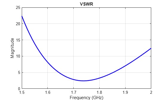
The VSWR of the antenna can be plotted using the function vswr used below. A VSWR value of 1.5:1 means that a maximum standing wave amplitude is 1.5 times greater than the minimum standing wave amplitude. The standing waves are generated because of impedance mismatch at the port. The VSWR is expressed through the reflection coefficient as .
figure
vswr(ant,freq);
Antenna Bandwidth
Bandwidth is a fundamental antenna parameter. The antenna bandwidth is the band of frequencies over which the antenna can properly radiate or receive power. Often, the desired bandwidth is one of the critical parameters used to decide an antenna type. Antenna bandwidth is usually the frequency band over which the magnitude of the reflection coefficient is below -10 dB, or the magnitude of the return loss is greater than 10 dB, or the VSWR is less than approximately 2. All these criteria are equivalent. We observe from the previous figures that the PIFA has no operating bandwidth in the frequency band of interest. The bandwidth is controlled by the proper antenna design. Sometimes, the reference impedance may be changed too. In the impedance plot we observe that the resistance of the present antenna is close to 20 at the resonance. Choose the reference impedance of 20 instead of 50 and plot the reflection coefficient.
S = sparameters(ant,freq,20);
figure
rfplot(S);
Now, we observe the reflection coefficient of less than -10 dB over the frequency band from 1.71 to 1.77 GHz. This is the antenna bandwidth. The same conclusion holds when using the VSWR or return loss calculations.
References
[1] C. A. Balanis, Antenna Theory. Analysis and Design, p. 514, Wiley, New York, 3rd Edition, 2005.
[2] T. S. Bird, "Definition and Misuse of Return Loss," Antennas and Propagation Magazine, April 2009.
See Also
Current Visualization on Antenna Surface | Analysis of Monopole Impedance