Matlab Euler-Lagrange Library

Using this library one can derive differential equations for any dynamic systems and solve response of the system for a given conditions.

Matlab: Euler-Lagrange Library for Derving Equations of Dynamic Systems

Using the above library, one can derive differential equations for any dynamic systems and solve response of the system for a given conditions.

Functionality of the library has been illustrated by the following examples:

1. Double Pendulum
2. Spring Pendulum
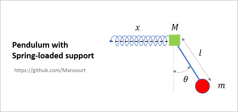
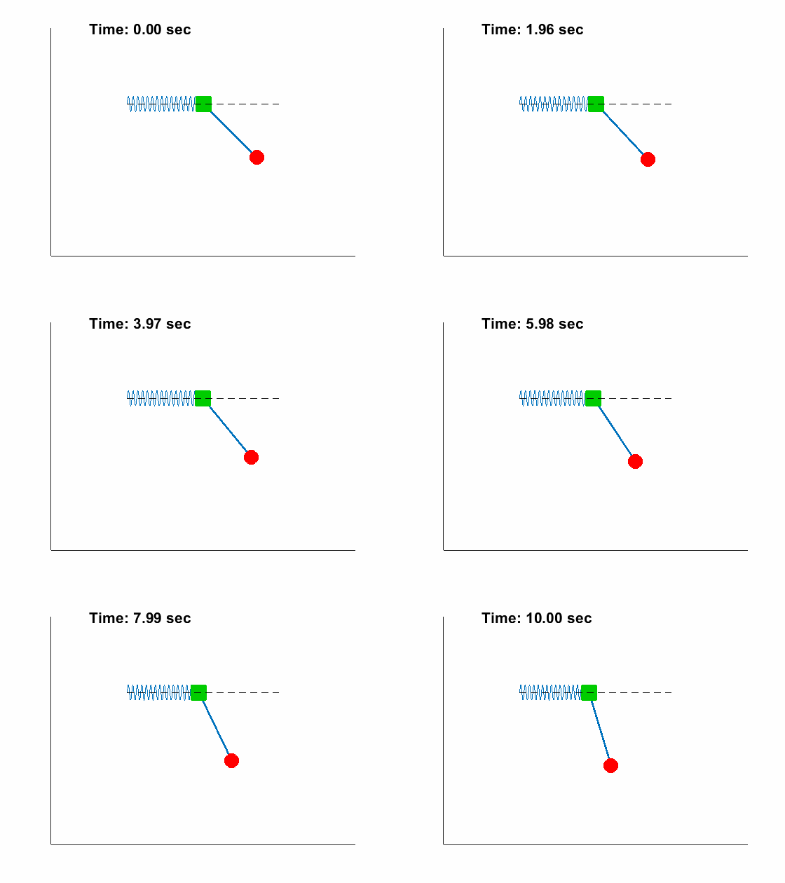
3. Pendulum with Spring-loaded support
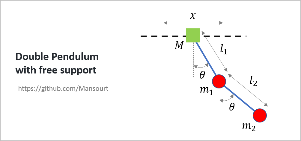
4. Double Pendulum with free support
5. Double Spring Pendulum
6. Coupled Pendulum
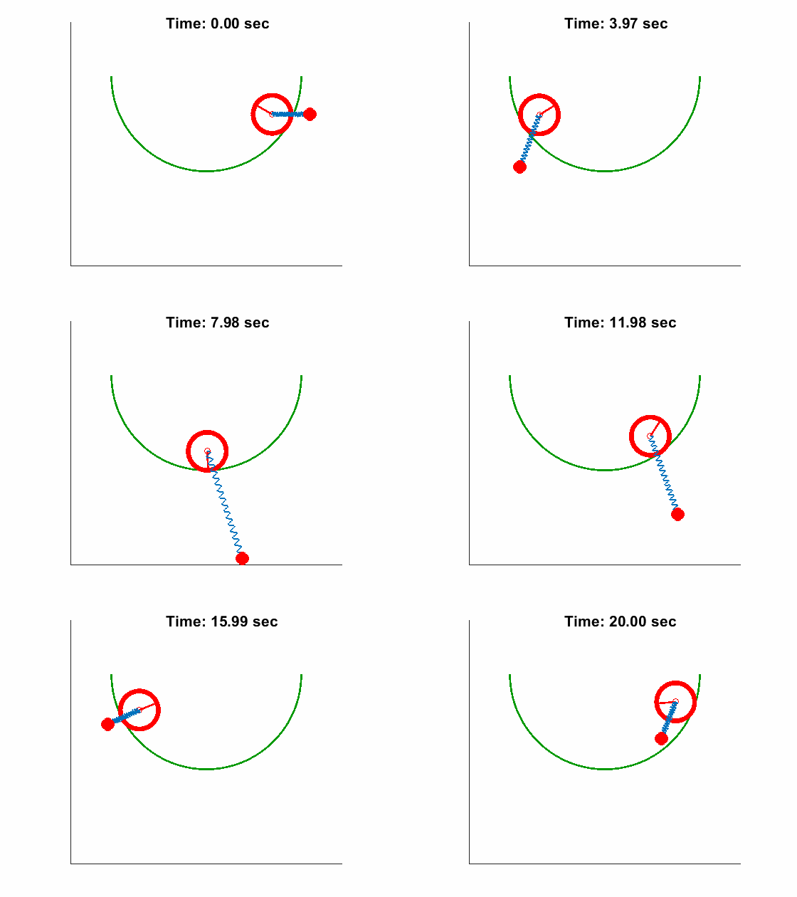
7. Spring Pendulum with Rolling base inside a semicircle

Example 1: Double Pendulum

Problem Definition:

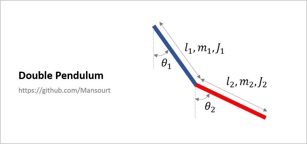
How to solve:

Just run the EVAL1.m to derive equations and solve intial condition problem:

Code Usage:

syms th1 th2  Dth1 Dth2 
syms l1 l2 m1 m2 J1 J2  g t 

%% Kinetic and Potential Energy
T1 = 1/2*J1*Dth1^2 + 1/2*m1*(l1/2*Dth1)^2;

Vc2_x = l1*Dth1*cos(th1) + l2/2*(Dth2)*cos(th2);
Vc2_y = l1*Dth1*sin(th1) + l2/2*(Dth2)*sin(th2);
Vc2 = sqrt(Vc2_x^2 + Vc2_y^2); 

T2 = 1/2*J2*(Dth2)^2 + 1/2*m2*Vc2^2;

T = T1 + T2;

V1 = m1*g*l1/2 * (1-cos(th1));
V2 = m2*g*(l1*(1-cos(th1)) + l2/2*(1-cos(th2)));
V = V1 + V2;

L = T - V;
%%
q  = [th1, th2];
Dq = [Dth1, Dth2];
tt = linspace(0,5,500);
Eq = LagrangeDynamicEqDeriver(L, q, Dq);
[SS, xx] = DynamicEqSolver(Eq, q, Dq, [l1 l2 m1 m2 J1 J2 g],...
                           [0.5, 0.5, 1, 5, 0.2, 0.5, 9.81], tt, [120,30,0,0]/180*pi);

Anlges of double pendulum:	Animated Response:

Watch on YouTube:

Example 2: Spring Pendulum

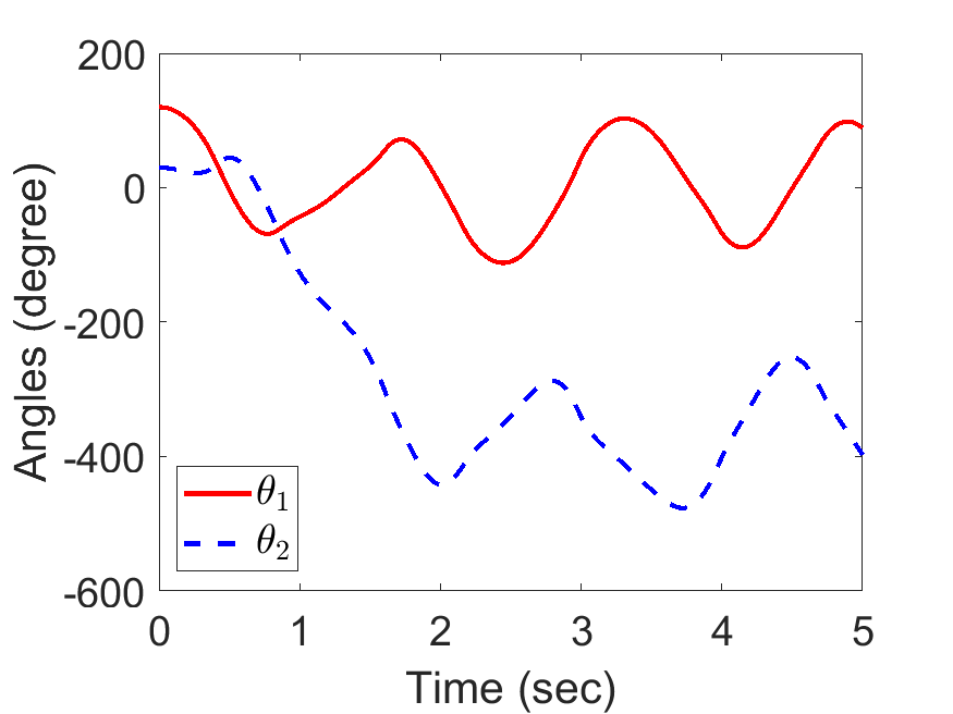
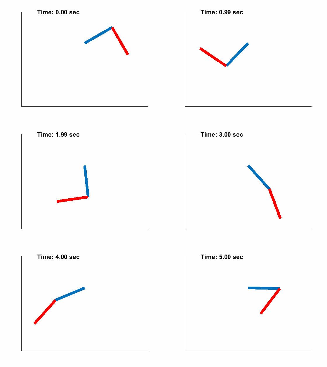
Problem Definition:

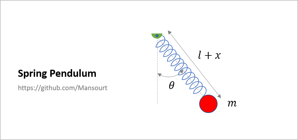
How to solve:

Just run the EVAL2.m to derive equations and solve intial condition problem:

Code Usage:

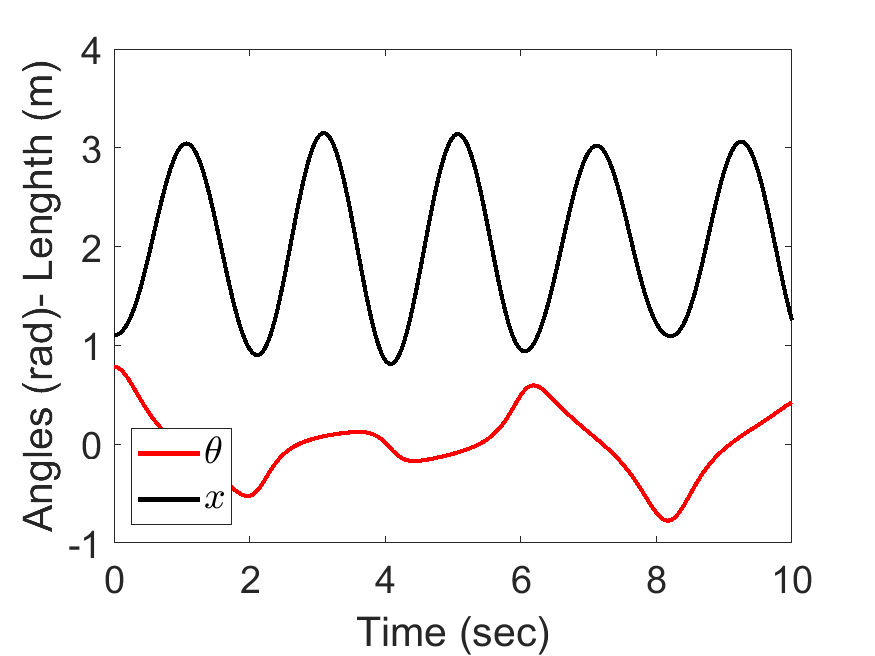
syms th Dth x Dx
syms m l k g t 

%% Kinetic and Potential Energy
T = 1/2*m*(Dx^2 + (l + x)^2*Dth^2);
V = -m*g*(l+x)*cos(th) + 1/2*k*x^2;

L = T - V;
%% Derive Equations
q = [th, x]; Dq = [Dth, Dx];
Eq = LagrangeDynamicEqDeriver(L, q, Dq);

%% Solve Equations

tt = linspace(0,10,300);
[SS, xx] = DynamicEqSolver(Eq, q, Dq, [m l k g],...
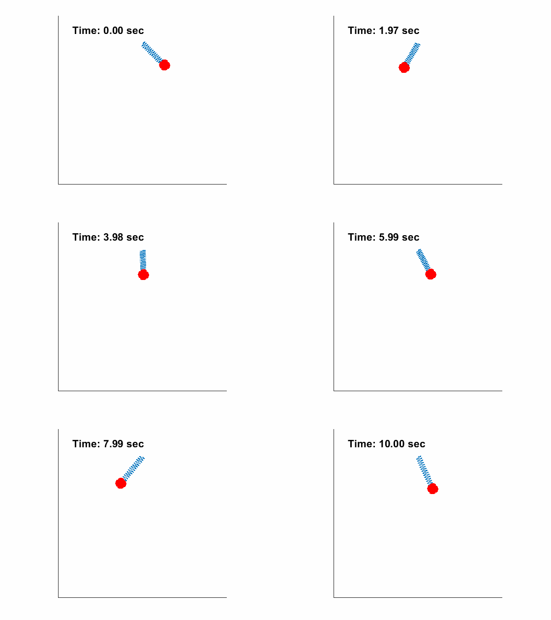
                           [1 1 10 9.81], tt, [45/180*pi,0.1, 0, 0]);

Angle and length of spring pendulum:	Animated Response:

Watch on YouTube:

Example 3: Pendulum with Spring-loaded support

Problem Definition:

How to solve:

Just run the EVAL3.m to derive equations and solve intial condition problem:

Code Usage:

syms th Dth x Dx
syms M m l k g 

%% Kinetic and Potential Energy
Vx2 = (Dx + l*Dth*cos(th))^2 + (l*Dth*sin(th))^2;
T   = 1/2*m*Vx2 + 1/2*M*Dx^2;

V = m*g*l*(1-cos(th)) + 1/2*k*x^2;

L = T - V;
%% Derive Equations
q = [th, x]; Dq = [Dth, Dx];
Eq = LagrangeDynamicEqDeriver(L, q, Dq);

%% Solve Equations

tt = linspace(0,10,200);
[SS, xx] = DynamicEqSolver(Eq, q, Dq, [M m l k g],...
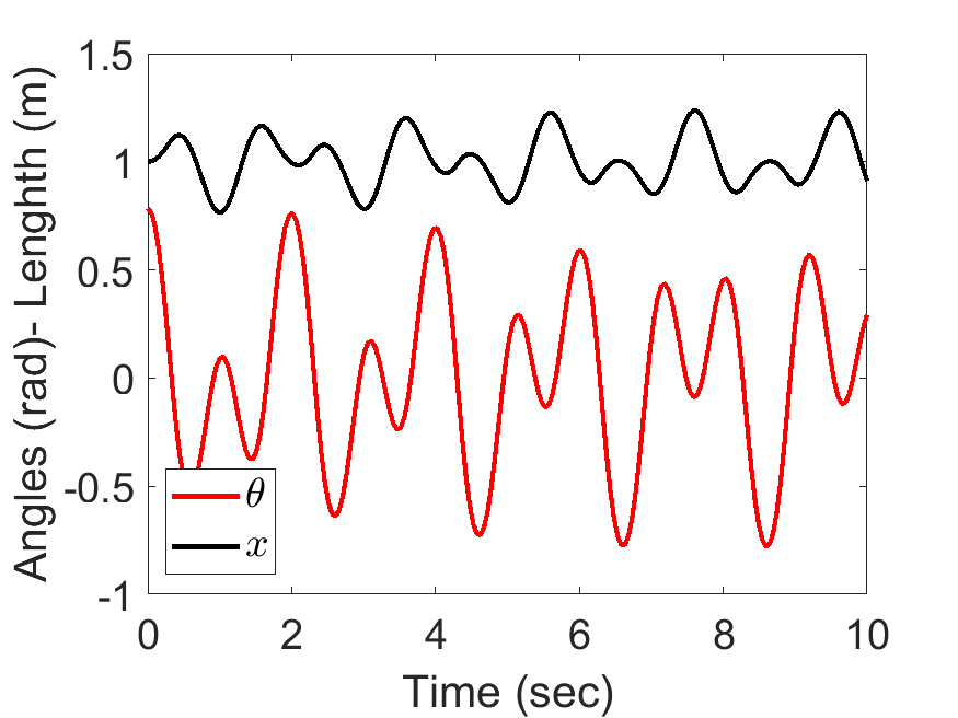
                           [2, 1, 0.5, 50, 9.81], tt, [45/180*pi,0, 0, 0]);

Slider Position and Pendulum Anlge:	Animated Response:

Watch on YouTube:

Example 4: Double Pendulum with free support

Problem Definition:

How to solve:

Just run the EVAL4.m to derive equations and solve intial condition problem:

Code Usage:

syms x th1 th2 Dx Dth1 Dth2 
syms M m1 m2 l1 l2 g

%% Kinetic and Potential Energy
v1x = l1*Dth1*cos(th1) + Dx;
v1y = l1*Dth1*sin(th1);

v2x = l1*Dth1*cos(th1) + l2*Dth2*cos(th2) + Dx;
v2y = l1*Dth1*sin(th1) + l2*Dth2*sin(th2);

v1t = v1x^2 + v1y^2; 
v2t = v2x^2 + v2y^2; 

T = 1/2*M*Dx^2 + 1/2*m1*v1t + 1/2*m2*v2t;

V1 = m1*g*l1*(1-cos(th1));
V2 = m2*g*(l1*(1-cos(th1))+l2*(1-cos(th2)));
V = V1 + V2;

L = T - V;
%%
q  = [x, th1, th2];
Dq = [Dx, Dth1, Dth2];
tt = linspace(0,25,500);
Eq = LagrangeDynamicEqDeriver(L, q, Dq);
[SS, xx] = DynamicEqSolver(Eq, q, Dq, [M m1 m2 l1 l2 g],...
                           [0.5, 0.5, 2, 1, 1, 9.81], tt, [0, pi/3, 2*pi/3, 0, 0, 0]);

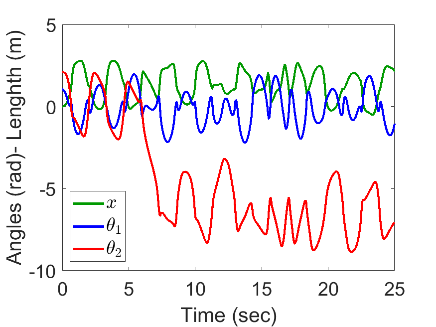
Slider Position, Pendulum Anlges:

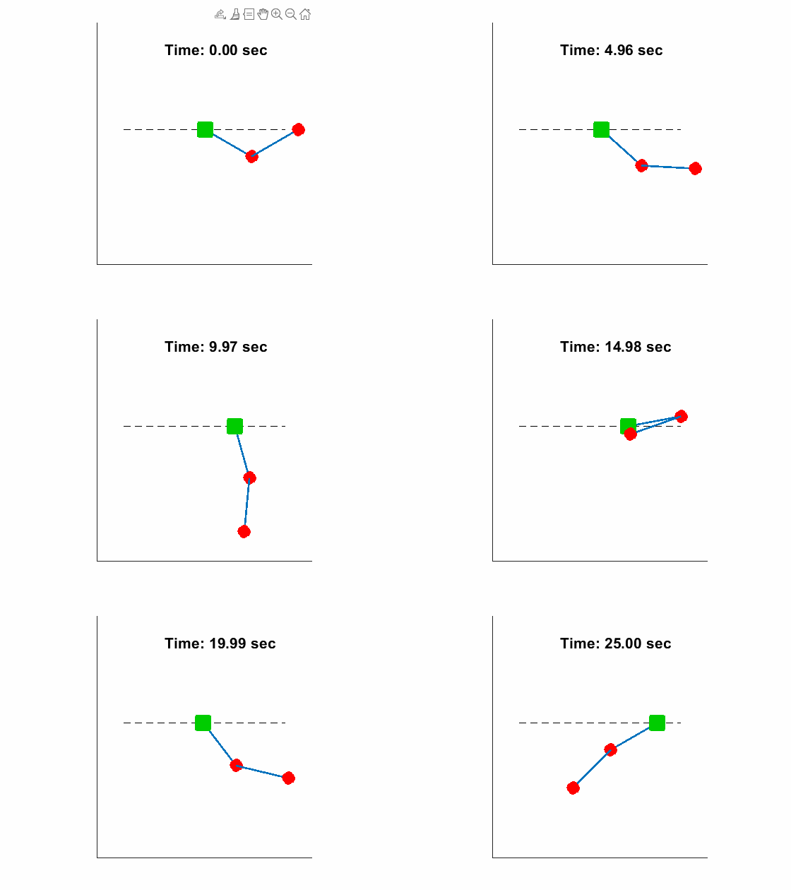
Slider Position, Pendulum Anlges:	Animated Response:

Watch on YouTube:

Example 5: Double Spring Pendulum

Problem Definition:

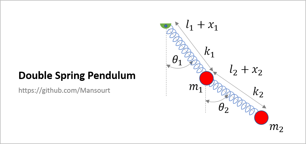
How to solve:

Just run the EVAL5.m to derive equations and solve intial condition problem:

Code Usage:

syms x1 x2 th1 th2 Dx1 Dx2 Dth1 Dth2 
syms k1 k2 m1 m2 l1 l2 g 

%% Kinetic and Potential Energy

v1x = Dx1*sin(th1) + (l1 + x1)*Dth1*cos(th1);
v1y = Dx1*cos(th1) - (l1 + x1)*Dth1*sin(th1);

v2x = Dx1*sin(th1) + (l1 + x1)*Dth1*cos(th1) + Dx2*sin(th2) + (l2 + x2)*Dth2*cos(th2);
v2y = Dx1*cos(th1) - (l1 + x1)*Dth1*sin(th1) + Dx2*cos(th2) - (l2 + x2)*Dth2*sin(th2);

v1t = v1x^2 + v1y^2; 
v2t = v2x^2 + v2y^2; 

T = 1/2*m1*v1t + 1/2*m2*v2t;

V1 = -m1*g*((l1 + x1)*cos(th1)) + 1/2*k1*x1^2;
V2 = -m2*g*((l1 + x1)*cos(th1) + (l2 + x2)*cos(th2)) + 1/2*k2*x2^2;
V = V1 + V2;

L = T - V;
%%
q  = [x1, x2, th1, th2];
Dq = [Dx1, Dx2, Dth1, Dth2];
tt = linspace(0, 15, 500);
Eq = LagrangeDynamicEqDeriver(L, q, Dq);
[SS, xx] = DynamicEqSolver(Eq, q, Dq, [k1 k2 m1 m2 l1 l2 g],...
                           [20, 100, 1, 2, 1, 1, 9.81], tt, [0, 0, pi/3, 2*pi/3, 0, 0, 0, 0]);

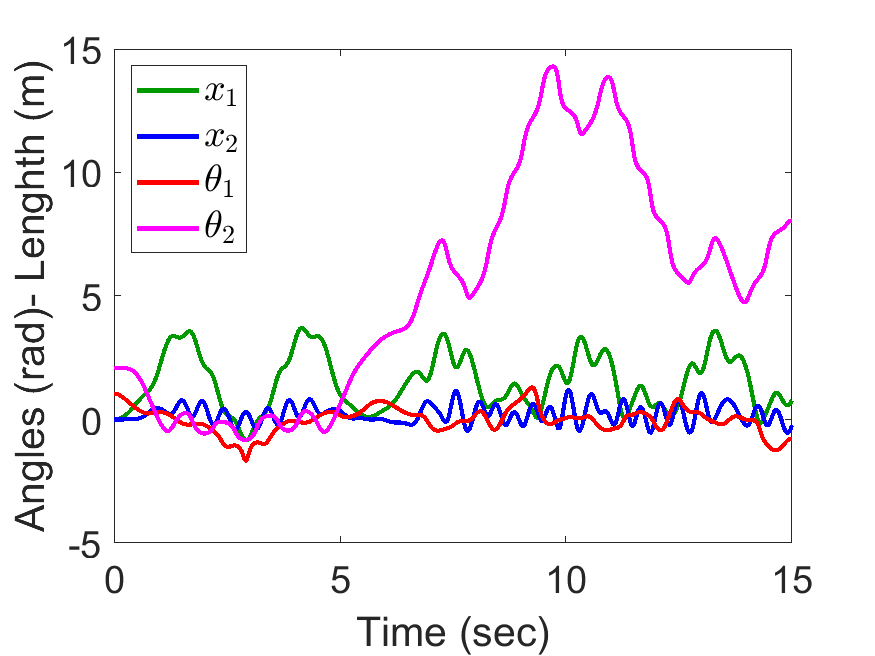
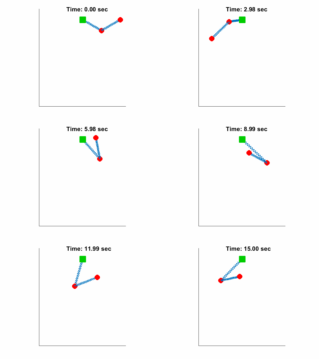
Slider Position, Pendulum Anlges:

Angle and length of spring pendulum:	Animated Response:

Watch on YouTube:

Example 6: Coupled Pendulum

Problem Definition:

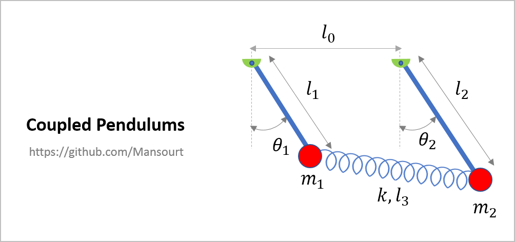
How to solve:

Just run the EVAL6.m to derive equations and solve intial condition problem:

Code Usage:

syms th1 th2 Dth1 Dth2 
syms k m1 m2 l0 l1 l2 l3 g 

%% Kinetic and Potential Energy

v1x = l1*Dth1*cos(th1) ;
v1y = -l1*Dth1*sin(th1);

v2x = l2*Dth2*cos(th2) ;
v2y = -l2*Dth2*sin(th2);

v1t = v1x^2 + v1y^2; 
v2t = v2x^2 + v2y^2; 

T = 1/2*m1*v1t + 1/2*m2*v2t;

dXX = l0 + l2*sin(th2) - l1*sin(th1);
dYY = l1*cos(th1) - l2*cos(th2);
dx = (dXX^2 + dYY^2)^0.5 - l3;

V1 = -m1*g*(l1*cos(th1)) + 1/2*k*dx^2;
V2 = -m2*g*(l2*cos(th2));
V = V1 + V2;

L = T - V;
%%
q  = [th1, th2];
Dq = [Dth1, Dth2];
tt = linspace(0, 20, 500);
Eq = LagrangeDynamicEqDeriver(L, q, Dq);
l0n = 2; l1n = 1; l2n = 1.5; l3n = 2;
[SS, xx] = DynamicEqSolver(Eq, q, Dq, [k m1 m2 l0 l1 l2 l3 g],...
                           [20,1,3, l0n, l1n, l2n, l3n, 9.81], tt, [pi/6, pi/2.5, 0, 0]);

Slider Position, Pendulum Anlges:

Angles of coupled pendulum:	Animated Response:

Example 7: Spring Pendulum with Rolling base inside a semicircle

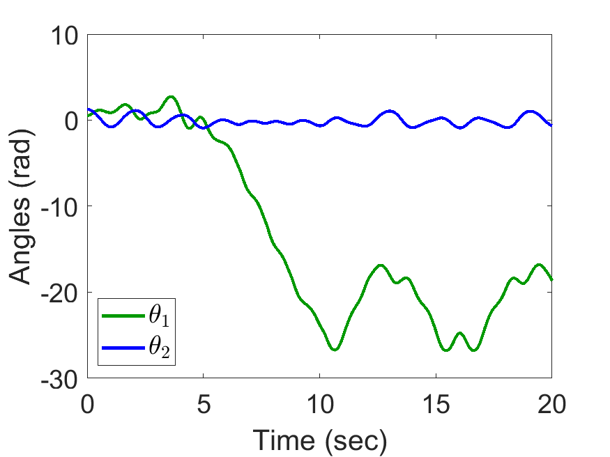
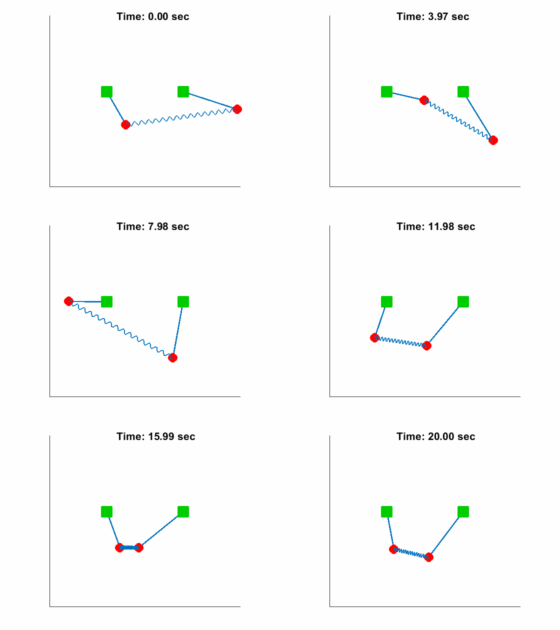
Problem Definition:

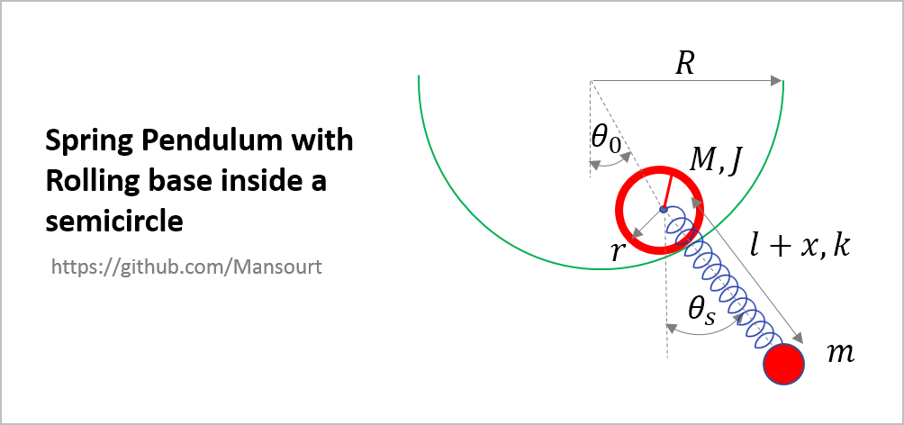
How to solve:

Just run the EVAL7.m to derive equations and solve intial condition problem:

Code Usage:

syms th0 ths x Dth0 Dths Dx
syms R r M J m k l g 

%% Kinetic and Potential Energy

VoM = (R-r)*[cos(th0), sin(th0)];
Wd  = -(R-r)*Dth0/r;

Vm = (R-r)*Dth0*[cos(th0), sin(th0)] + (l+x)*Dths*[cos(ths), sin(ths)] + Dx*[sin(ths), -cos(ths)];

yM = -(R-r)*cos(th0);
ym = yM - (l+x)*cos(ths);

T = 1/2*M*(VoM*VoM.') + 1/2*m*(Vm*Vm.') + 1/2*J*Wd^2;

V = M*g*yM + m*g*ym + 1/2*k*x^2;

L = T - V;
%%
q  = [th0, ths, x];
Dq = [Dth0, Dths, Dx];
tt = linspace(0, 20, 500);
Eq = LagrangeDynamicEqDeriver(L, q, Dq);
R0 = 5; r0 = 1; l0 = 2; 
[SS, xx] = DynamicEqSolver(Eq, q, Dq, [R r M J m k l g],...
                           [R0, r0, 1, 2, 3, 30, l0, 9.81], tt, [pi/3, pi/2, 0, 0, 0, 0]);

Slider Position, Pendulum Anlges:

Angles of spring length:	Animated Response:

Example 8: Coupled Triple Pendulums with Spring-loaded sliding support

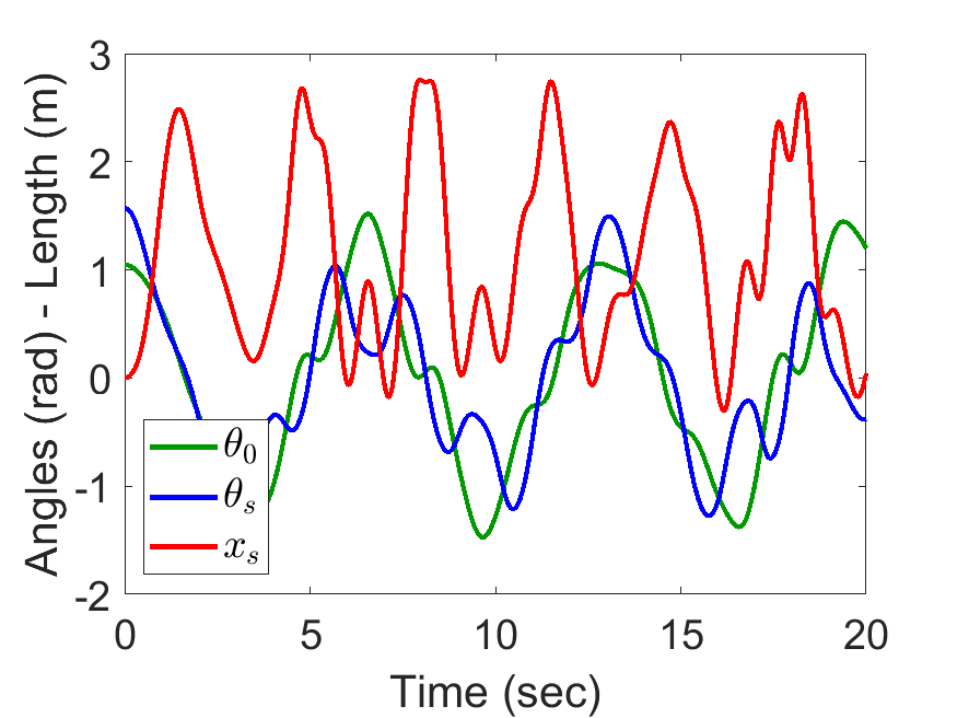
Problem Definition:

Simulation Results:

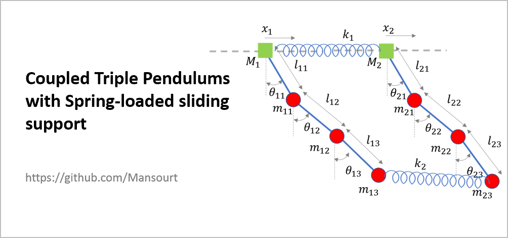
The simulation results are based on the following Values:

% List of Parameter Values
Plist1 = [M1 m11 m12 m13 l11 l12 l13];
Pval1  = [4, 2, 1,1, 1, 1,1];
Plist2 = [M2 m21 m22 m23 l21 l22 l23];
Pval2  = [8, 2, 1,1, 1, 1,1];

Plist3 = [g l0 ls1 ls2 k1 k2];
Pval3  = [9.8, 1, 1,1, 100,50];

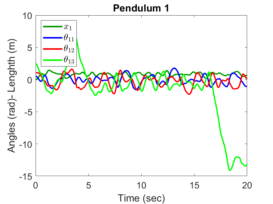
% Initial Conditions
x01  = [0,pi/6,2*pi/6,4*pi/5];
Dx01 = zeros(1,4);
x02  = [0.5,pi/4,2*pi/4,5*pi/8];
Dx02 = zeros(1,4);

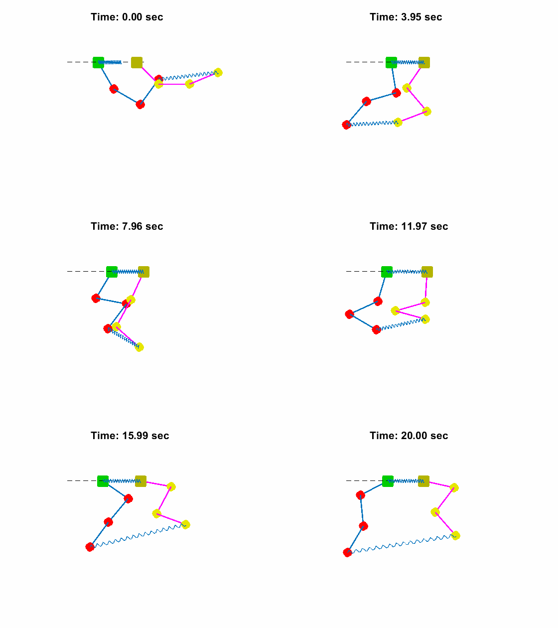
Triple Pendulum #1 Position and Anlges:

Triple Pendulum #1 Position and Anlges:	Animated Response:

Example 9: Spherical Pendulum (3D)

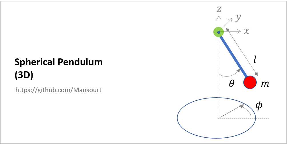
Problem Definition:

Simulation Results:

The simulation results are based on the following Values:

% List of Parameter Values
m0 = 1;
l0 = 2;
g0 = 9.81;

% Initial Conditions
th0  = 50;
phi0 = 0;
Dth0 = 0;
Dphi0 = 75;

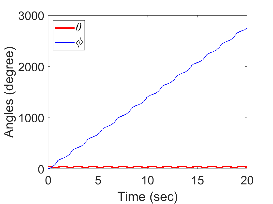
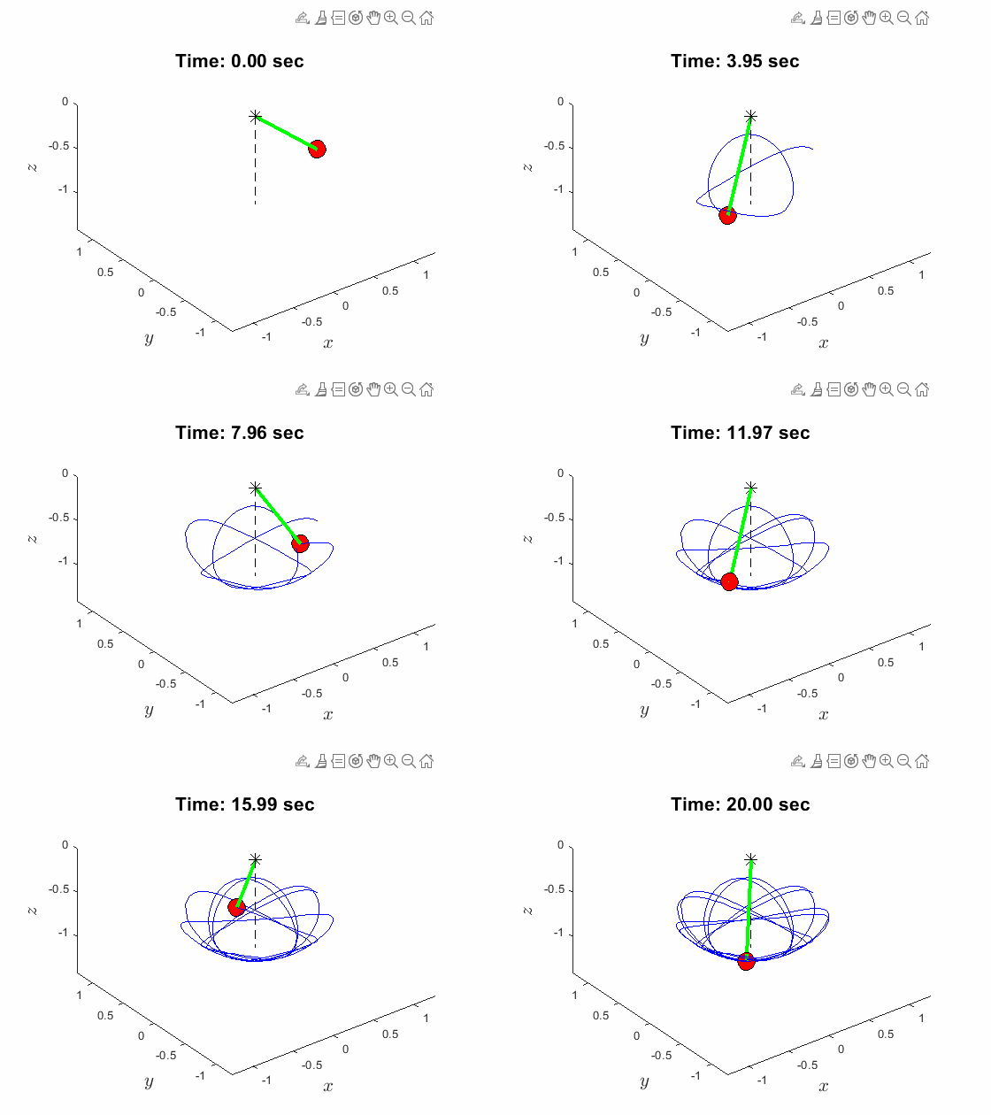
Spherical Pendulum Anlges:

Spherical Pendulum Anlges:	Animated Response:

Contact

Email: [e-mail] | [e-mail]