Ergebnisse für
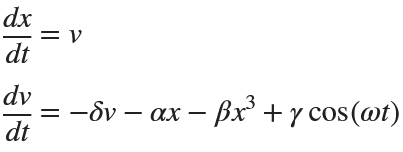
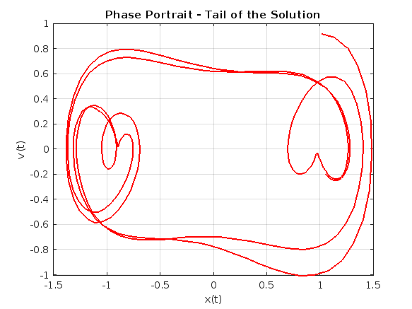
Following on from my previous post The Non-Chaotic Duffing Equation, now we will study the chaotic behaviour of the Duffing Equation
P.s:Any comments/advice on improving the code is welcome.
The Original Duffing Equation is the following:
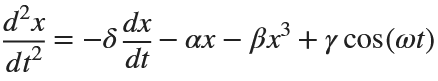
Let 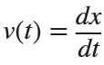 . This implies that
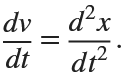
Then we rewrite it as a System of First-Order Equations
Using the substitution  for
for  , the second-order equation can be transformed into the following system of first-order equations:
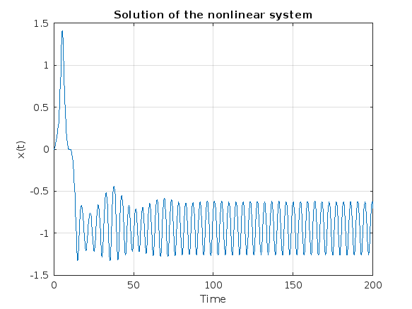
Exploring the Effect of γ.
% Define parameters
gamma = 0.1;
alpha = -1;
beta = 1;
delta = 0.1;
omega = 1.4;
% Define the system of equations
odeSystem = @(t, y) [y(2);
-delta*y(2) - alpha*y(1) - beta*y(1)^3 + gamma*cos(omega*t)];
% Initial conditions
y0 = [0; 0]; % x(0) = 0, v(0) = 0
% Time span
tspan = [0 200];
% Solve the system
[t, y] = ode45(odeSystem, tspan, y0);
% Plot the results
figure;
plot(t, y(:, 1));
xlabel('Time');
ylabel('x(t)');
title('Solution of the nonlinear system');
grid on;
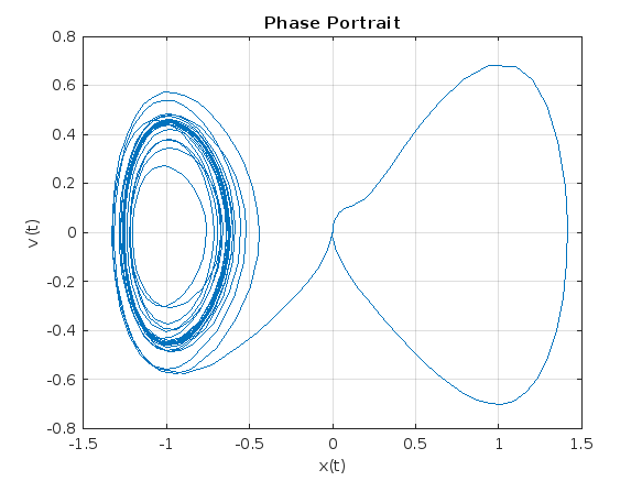
% Plot the phase portrait
figure;
plot(y(:, 1), y(:, 2));
xlabel('x(t)');
ylabel('v(t)');
title('Phase Portrait');
grid on;
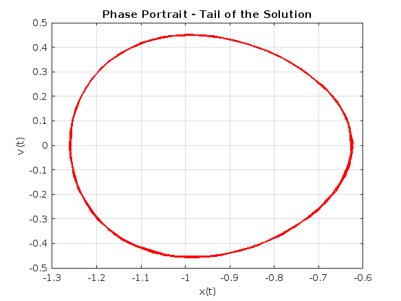
% Define the tail (e.g., last 10% of the time interval)
tail_start = floor(0.9 * length(t)); % Starting index for the tail
tail_end = length(t); % Ending index for the tail
% Plot the tail of the solution
figure;
plot(y(tail_start:tail_end, 1), y(tail_start:tail_end, 2), 'r', 'LineWidth', 1.5);
xlabel('x(t)');
ylabel('v(t)');
title('Phase Portrait - Tail of the Solution');
grid on;
% Define parameters
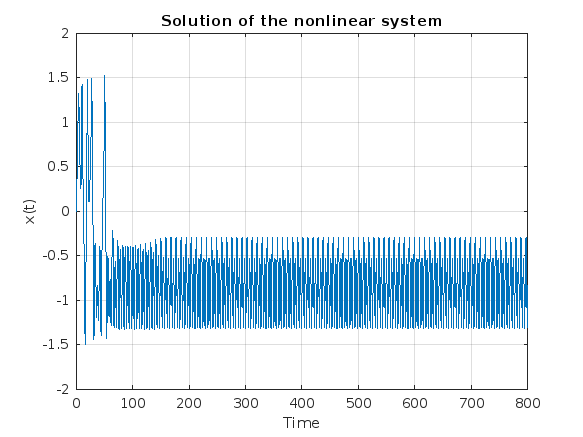
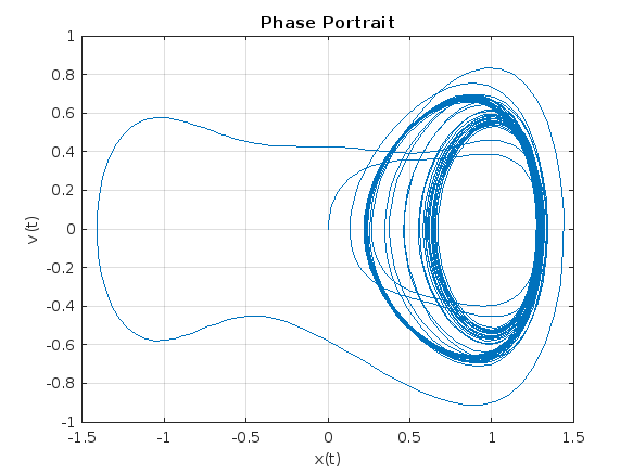
gamma = 0.318;
alpha = -1;
beta = 1;
delta = 0.1;
omega = 1.4;
% Define the system of equations
odeSystem = @(t, y) [y(2);
-delta*y(2) - alpha*y(1) - beta*y(1)^3 + gamma*cos(omega*t)];
% Initial conditions
y0 = [0; 0]; % x(0) = 0, v(0) = 0
% Time span
tspan = [0 800];
% Solve the system
[t, y] = ode45(odeSystem, tspan, y0);
% Plot the results
figure;
plot(t, y(:, 1));
xlabel('Time');
ylabel('x(t)');
title('Solution of the nonlinear system');
grid on;
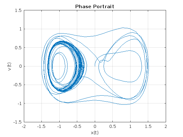
% Plot the phase portrait
figure;
plot(y(:, 1), y(:, 2));
xlabel('x(t)');
ylabel('v(t)');
title('Phase Portrait');
grid on;
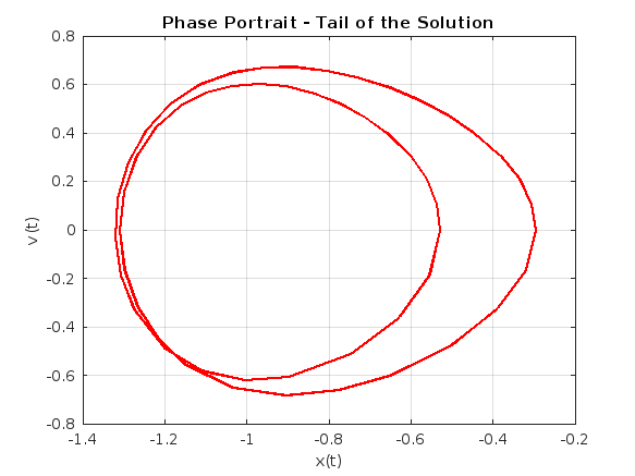
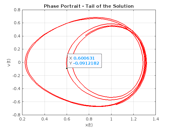
% Define the tail (e.g., last 10% of the time interval)
tail_start = floor(0.9 * length(t)); % Starting index for the tail
tail_end = length(t); % Ending index for the tail
% Plot the tail of the solution
figure;
plot(y(tail_start:tail_end, 1), y(tail_start:tail_end, 2), 'r', 'LineWidth', 1.5);
xlabel('x(t)');
ylabel('v(t)');
title('Phase Portrait - Tail of the Solution');
grid on;
% Define parameters
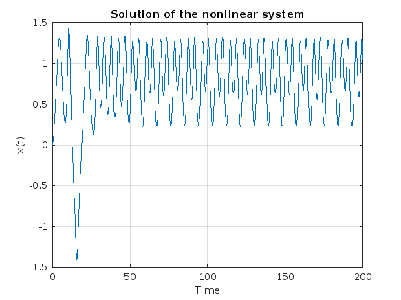
gamma = 0.338;
alpha = -1;
beta = 1;
delta = 0.1;
omega = 1.4;
% Define the system of equations
odeSystem = @(t, y) [y(2);
-delta*y(2) - alpha*y(1) - beta*y(1)^3 + gamma*cos(omega*t)];
% Initial conditions
y0 = [0; 0]; % x(0) = 0, v(0) = 0
% Time span with more points for better resolution
tspan = linspace(0, 200,2000); % Increase the number of points
% Solve the system
[t, y] = ode45(odeSystem, tspan, y0);
% Plot the results
figure;
plot(t, y(:, 1));
xlabel('Time');
ylabel('x(t)');
title('Solution of the nonlinear system');
grid on;
% Plot the phase portrait
figure;
plot(y(:, 1), y(:, 2));
xlabel('x(t)');
ylabel('v(t)');
title('Phase Portrait');
grid on;
% Define the tail (e.g., last 10% of the time interval)
tail_start = floor(0.9 * length(t)); % Starting index for the tail
tail_end = length(t); % Ending index for the tail
% Plot the tail of the solution
figure;
plot(y(tail_start:tail_end, 1), y(tail_start:tail_end, 2), 'r', 'LineWidth', 1.5);
xlabel('x(t)');
ylabel('v(t)');
title('Phase Portrait - Tail of the Solution');
grid on;
ax = gca;
chart = ax.Children(1);
datatip(chart,0.5581,-0.1126);
% Define parameters
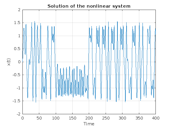
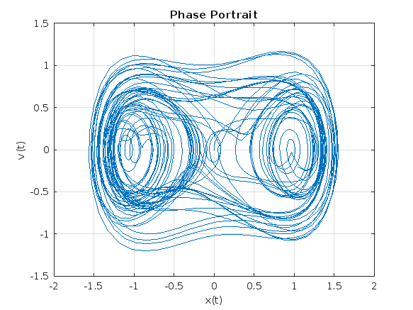
gamma = 0.35;
alpha = -1;
beta = 1;
delta = 0.1;
omega = 1.4;
% Define the system of equations
odeSystem = @(t, y) [y(2);
-delta*y(2) - alpha*y(1) - beta*y(1)^3 + gamma*cos(omega*t)];
% Initial conditions
y0 = [0; 0]; % x(0) = 0, v(0) = 0
% Time span with more points for better resolution
tspan = linspace(0, 400,3000); % Increase the number of points
% Solve the system
[t, y] = ode45(odeSystem, tspan, y0);
% Plot the results
figure;
plot(t, y(:, 1));
xlabel('Time');
ylabel('x(t)');
title('Solution of the nonlinear system');
grid on;
% Plot the phase portrait
figure;
plot(y(:, 1), y(:, 2));
xlabel('x(t)');
ylabel('v(t)');
title('Phase Portrait');
grid on;
% Define the tail (e.g., last 10% of the time interval)
tail_start = floor(0.9 * length(t)); % Starting index for the tail
tail_end = length(t); % Ending index for the tail
% Plot the tail of the solution
figure;
plot(y(tail_start:tail_end, 1), y(tail_start:tail_end, 2), 'r', 'LineWidth', 1.5);
xlabel('x(t)');
ylabel('v(t)');
title('Phase Portrait - Tail of the Solution');
grid on;
Studying the attached document Duffing Equation from the University of Colorado, I noticed that there is an analysis of The Non-Chaotic Duffing Equation and all the graphs were created with Matlab. And since the code is not given I took the initiative to try to create the same graphs with the following code.
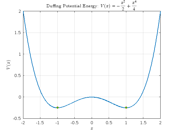
- Plotting the Potential Energy and Identifying Extrema
% Define the range of x values
x = linspace(-2, 2, 1000);
% Define the potential function V(x)
V = -x.^2 / 2 + x.^4 / 4;
% Plot the potential function
figure;
plot(x, V, 'LineWidth', 2);
hold on;
% Mark the minima at x = ±1
plot([-1, 1], [-1/4, -1/4], 'ro', 'MarkerSize', 5, 'MarkerFaceColor', 'g');
% Add LaTeX title and labels
title('Duffing Potential Energy: $$V(x) = -\frac{x^2}{2} + \frac{x^4}{4}$$', 'Interpreter', 'latex');
xlabel('$$x$$', 'Interpreter', 'latex');
ylabel('$$V(x)$$','Interpreter', 'latex');
grid on;
hold off;
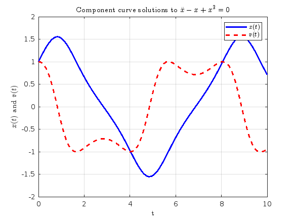
- Solving and Plotting the Duffing Equation
% Define the system of ODEs for the non-chaotic Duffing equation
duffing_ode = @(t, X) [X(2);
X(1) - X(1).^3];
% Time span for the simulation
tspan = [0 10];
% Initial conditions [x(0), v(0)]
initial_conditions = [1; 1];
% Solve the ODE using ode45
[t, X] = ode45(duffing_ode, tspan, initial_conditions);
% Extract displacement (x) and velocity (v)
x = X(:, 1);
v = X(:, 2);
% Plot both x(t) and v(t) in the same figure
figure;
plot(t, x, 'b-', 'LineWidth', 2); % Plot x(t) with blue line
hold on;
plot(t, v, 'r--', 'LineWidth', 2); % Plot v(t) with red dashed line
% Add title, labels, and legend
title(' Component curve solutions to $$\ddot{x}-x+x^3=0$$','Interpreter', 'latex');
xlabel('t','Interpreter', 'latex');
ylabel('$$x(t) $$ and $$v(t) $$','Interpreter', 'latex');
legend('$$x(t)$$', ' $$v(t)$$','Interpreter', 'latex');
grid on;
hold off;
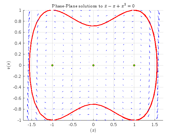
% Phase portrait with nullclines, equilibria, and vector field
figure;
hold on;
% Plot phase portrait
plot(x, v,'r', 'LineWidth', 2);
% Plot equilibrium points
plot([0 1 -1], [0 0 0], 'ro', 'MarkerSize', 5, 'MarkerFaceColor', 'g');
% Create a grid of points for the vector field
[x_vals, v_vals] = meshgrid(linspace(-2, 2, 20), linspace(-1, 1, 20));
% Compute the vector field components
dxdt = v_vals;
dvdt = x_vals - x_vals.^3;
% Plot the vector field
quiver(x_vals, v_vals, dxdt, dvdt, 'b');
% Set axis limits to [-1, 1]
xlim([-1.7 1.7]);
ylim([-1 1]);
% Labels and title
title('Phase-Plane solutions to $$\ddot{x}-x+x^3=0$$','Interpreter', 'latex');
xlabel('$$ (x)$$','Interpreter', 'latex');
ylabel('$$v(v)$$','Interpreter', 'latex');
grid on;
hold off;