Hauptinhalt
Ergebnisse für
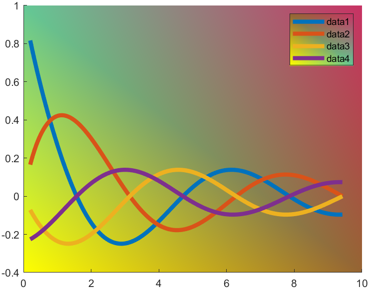
t=0.2:0.01:3*pi;
hold on
plot(t,cos(t)./(1+t),'LineWidth',4)
plot(t,sin(t)./(1+t),'LineWidth',4)
plot(t,cos(t+pi/2)./(1+t+pi/2),'LineWidth',4)
plot(t,cos(t+pi)./(1+t+pi),'LineWidth',4)
ax=gca;
hLegend=legend();
pause(1e-16)
colorData = uint8([255, 150, 200, 100; ...
255, 100, 50, 200; ...
0, 50, 100, 150; ...
102, 150, 200, 50]);
set(ax.Backdrop.Face, 'ColorBinding','interpolated','ColorData',colorData);
set(hLegend.BoxFace,'ColorBinding','interpolated','ColorData',colorData)
I have written two tools and uploaded fileexchange, which allows us to easily draw chord diagrams:
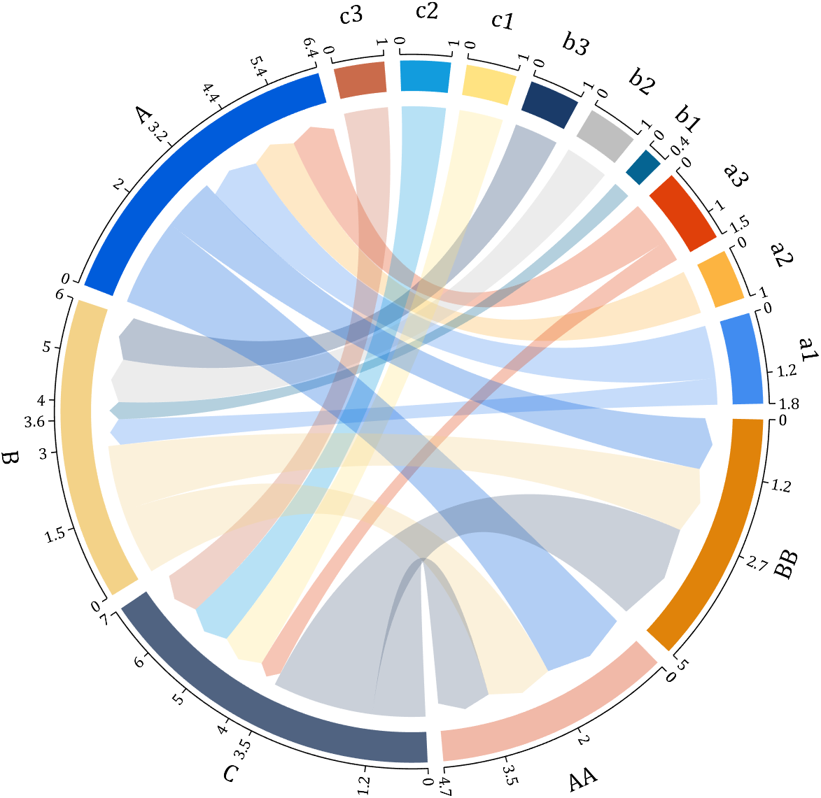

chord chart 弦图
download:
demo:
dataMat=[2 0 1 2 5 1 2;
3 5 1 4 2 0 1;
4 0 5 5 2 4 3];
dataMat=dataMat+rand(3,7);
dataMat(dataMat<1)=0;
colName={'G1','G2','G3','G4','G5','G6','G7'};
rowName={'S1','S2','S3'};
CC=chordChart(dataMat,'rowName',rowName,'colName',colName);
CC=CC.draw();
CC.setFont('FontSize',17,'FontName','Cambria')
% 显示刻度和数值
% Displays scales and numeric values
CC.tickState('on')
CC.tickLabelState('on')
% 调节标签半径
% Adjustable Label radius
CC.setLabelRadius(1.4);

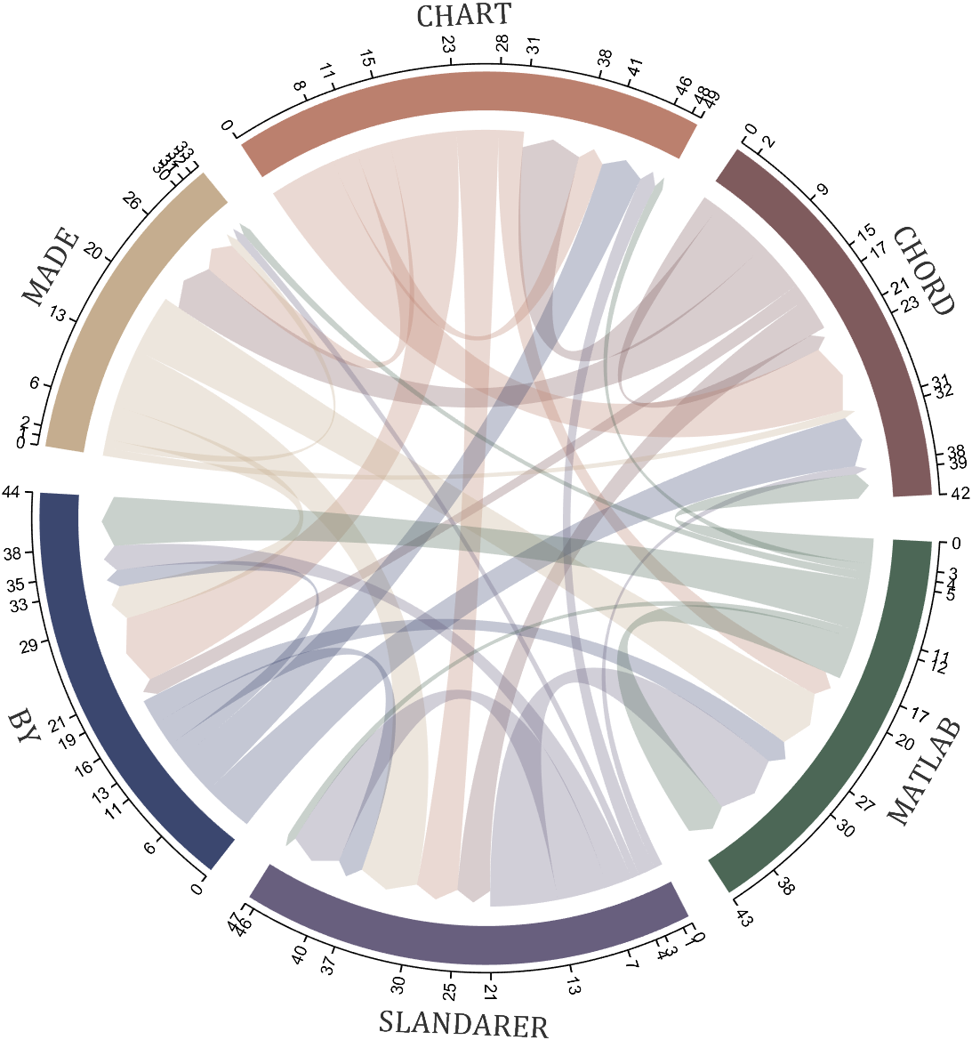
Digraph chord chart 有向弦图
download:
demo:
dataMat=randi([0,8],[6,6]);
% 添加标签名称
NameList={'CHORD','CHART','MADE','BY','SLANDARER','MATLAB'};
BCC=biChordChart(dataMat,'Label',NameList,'Arrow','on');
BCC=BCC.draw();
% 添加刻度
BCC.tickState('on')
% 修改字体,字号及颜色
BCC.setFont('FontName','Cambria','FontSize',17,'Color',[.2,.2,.2])
BCC.setLabelRadius(1.3);
BCC.tickLabelState('on')
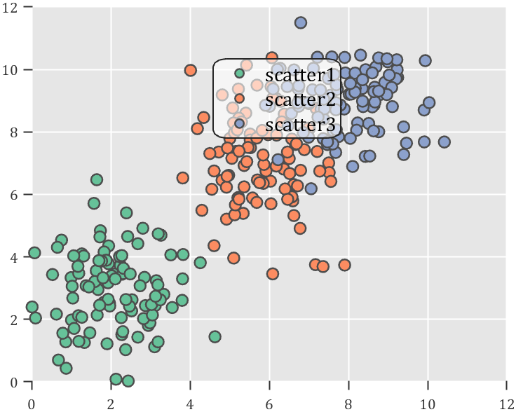
How to create a legend as follows?

Principle Explanation - Graphic Objects
Hidden Properties of Legend are laid as follows
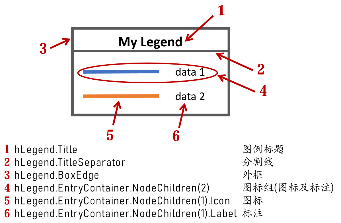
In most cases, legends are drawn using LineLoop and Quadrilateral:
Both of these basic graphic objects are drawn in groups of four points, and the general principle is as follows:

Of course, you can arrange the points in order, or set VertexIndices whitch means the vertex order to obtain the desired quadrilateral shape:

Other objects
Compared to objects that can only be grouped into four points, we also need to introduce more flexible objects. Firstly, LineStrip, a graphical object that draws lines in groups of two points:
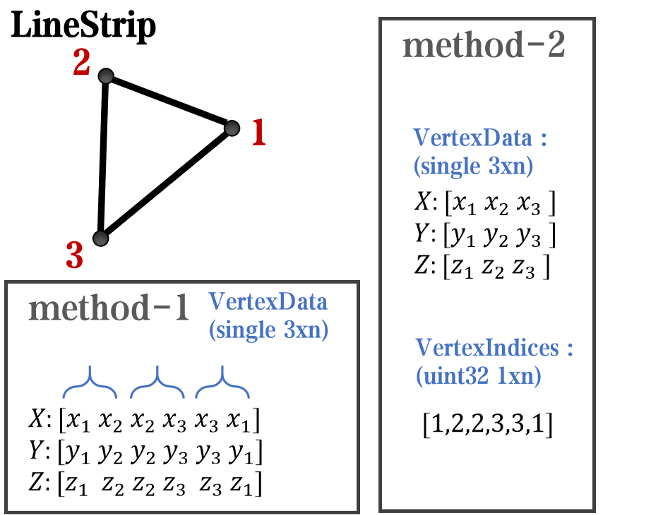
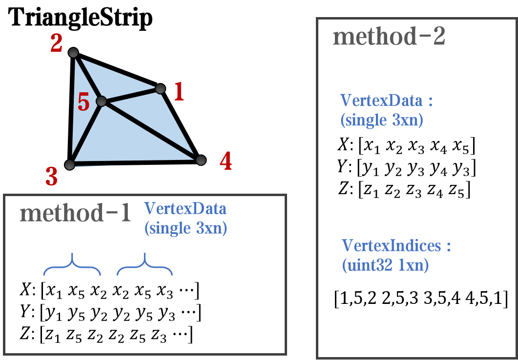
And TriangleStrip is a set of three points that draw objects to fill triangles, for example, complex polygons can be filled with multiple triangles:
Principle Explanation - Create and Replace
Let's talk about how to construct basic graphic objects, which are all constructed using undisclosed and very low-level functions, such as LineStrip, not through:
- LineStrip()
It is built through:
- matlab.graphics.primitive.world.LineStrip()
After building the object, the following properties must be set to make the hidden object visible:
- Layer
- ColorBinding
- ColorData
- VertexData
- PickableParts
The settings of these properties can refer to the original legend to form the object, which will not be elaborated here. You can also refer to the code I wrote.
Afterwards, set the newly constructed object's parent class as the Group parent class of the original component, and then hide the original component
newBoxEdgeHdl.Parent=oriBoxEdgeHdl.Parent;
oriBoxEdgeHdl.Visible='off';
The above is the entire process of component replacement, with two example codes written:
Semi transparent legend
function SPrettyLegend(lgd)
% Semitransparent rounded rectangle legend
% Copyright (c) 2023, Zhaoxu Liu / slandarer
% -------------------------------------------------------------------------
% Zhaoxu Liu / slandarer (2023). pretty legend
% (https://www.mathworks.com/matlabcentral/fileexchange/132128-pretty-legend),
% MATLAB Central File Exchange. 检索来源 2023/7/9.
% =========================================================================
if nargin<1
ax = gca;
lgd = get(ax,'Legend');
end
pause(1e-6)
Ratio = .1;
t1 = linspace(0,pi/2,4); t1 = t1([1,2,2,3,3,4]);
t2 = linspace(pi/2,pi,4); t2 = t2([1,2,2,3,3,4]);
t3 = linspace(pi,3*pi/2,4); t3 = t3([1,2,2,3,3,4]);
t4 = linspace(3*pi/2,2*pi,4); t4 = t4([1,2,2,3,3,4]);
XX = [1,1,1-Ratio+cos(t1).*Ratio,1-Ratio,Ratio,Ratio+cos(t2).*Ratio,...
0,0,Ratio+cos(t3).*Ratio,Ratio,1-Ratio,1-Ratio+cos(t4).*Ratio];
YY = [Ratio,1-Ratio,1-Ratio+sin(t1).*Ratio,1,1,1-Ratio+sin(t2).*Ratio,...
1-Ratio,Ratio,Ratio+sin(t3).*Ratio,0,0,Ratio+sin(t4).*Ratio];
% 圆角边框(border-radius)
oriBoxEdgeHdl = lgd.BoxEdge;
newBoxEdgeHdl = matlab.graphics.primitive.world.LineStrip();
newBoxEdgeHdl.AlignVertexCenters = 'off';
newBoxEdgeHdl.Layer = 'front';
newBoxEdgeHdl.ColorBinding = 'object';
newBoxEdgeHdl.LineWidth = 1;
newBoxEdgeHdl.LineJoin = 'miter';
newBoxEdgeHdl.WideLineRenderingHint = 'software';
newBoxEdgeHdl.ColorData = uint8([38;38;38;0]);
newBoxEdgeHdl.VertexData = single([XX;YY;XX.*0]);
newBoxEdgeHdl.Parent=oriBoxEdgeHdl.Parent;
oriBoxEdgeHdl.Visible='off';
% 半透明圆角背景(Semitransparent rounded background)
oriBoxFaceHdl = lgd.BoxFace;
newBoxFaceHdl = matlab.graphics.primitive.world.TriangleStrip();
Ind = [1:(length(XX)-1);ones(1,length(XX)-1).*(length(XX)+1);2:length(XX)];
Ind = Ind(:).';
newBoxFaceHdl.PickableParts = 'all';
newBoxFaceHdl.Layer = 'back';
newBoxFaceHdl.ColorBinding = 'object';
newBoxFaceHdl.ColorType = 'truecoloralpha';
newBoxFaceHdl.ColorData = uint8(255*[1;1;1;.6]);
newBoxFaceHdl.VertexData = single([XX,.5;YY,.5;XX.*0,0]);
newBoxFaceHdl.VertexIndices = uint32(Ind);
newBoxFaceHdl.Parent = oriBoxFaceHdl.Parent;
oriBoxFaceHdl.Visible = 'off';
end
Usage examples
clc; clear; close all
rng(12)
% 生成随机点(Generate random points)
mu = [2 3; 6 7; 8 9];
S = cat(3,[1 0; 0 2],[1 0; 0 2],[1 0; 0 1]);
r1 = abs(mvnrnd(mu(1,:),S(:,:,1),100));
r2 = abs(mvnrnd(mu(2,:),S(:,:,2),100));
r3 = abs(mvnrnd(mu(3,:),S(:,:,3),100));
% 绘制散点图(Draw scatter chart)
hold on
propCell = {'LineWidth',1.2,'MarkerEdgeColor',[.3,.3,.3],'SizeData',60};
scatter(r1(:,1),r1(:,2),'filled','CData',[0.40 0.76 0.60],propCell{:});
scatter(r2(:,1),r2(:,2),'filled','CData',[0.99 0.55 0.38],propCell{:});
scatter(r3(:,1),r3(:,2),'filled','CData',[0.55 0.63 0.80],propCell{:});
% 增添图例(Draw legend)
lgd = legend('scatter1','scatter2','scatter3');
lgd.Location = 'northwest';
lgd.FontSize = 14;
% 坐标区域基础修饰(Axes basic decoration)
ax=gca; grid on
ax.FontName = 'Cambria';
ax.Color = [0.9,0.9,0.9];
ax.Box = 'off';
ax.TickDir = 'out';
ax.GridColor = [1 1 1];
ax.GridAlpha = 1;
ax.LineWidth = 1;
ax.XColor = [0.2,0.2,0.2];
ax.YColor = [0.2,0.2,0.2];
ax.TickLength = [0.015 0.025];
% 隐藏轴线(Hide XY-Ruler)
pause(1e-6)
ax.XRuler.Axle.LineStyle = 'none';
ax.YRuler.Axle.LineStyle = 'none';
SPrettyLegend(lgd)
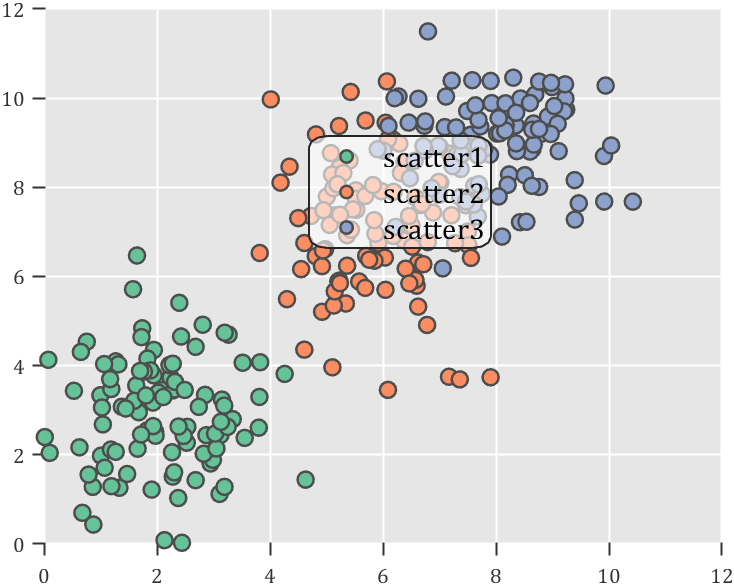
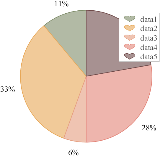
Heart shaped legend (exclusive to pie charts)
function pie2HeartLegend(lgd)
% Heart shaped legend for pie chart
% Copyright (c) 2023, Zhaoxu Liu / slandarer
% -------------------------------------------------------------------------
% Zhaoxu Liu / slandarer (2023). pretty legend
% (https://www.mathworks.com/matlabcentral/fileexchange/132128-pretty-legend),
% MATLAB Central File Exchange. 检索来源 2023/7/9.
% =========================================================================
if nargin<1
ax = gca;
lgd = get(ax,'Legend');
end
pause(1e-6)
% 心形曲线(Heart curve)
x = -1:1/100:1;
y1 = 0.6 * abs(x) .^ 0.5 + ((1 - x .^ 2) / 2) .^ 0.5;
y2 = 0.6 * abs(x) .^ 0.5 - ((1 - x .^ 2) / 2) .^ 0.5;
XX = [x, flip(x),x(1)]./3.4+.5;
YY = ([y1, y2,y1(1)]-.2)./2+.5;
Ind = [1:(length(XX)-1);2:length(XX)];
Ind = Ind(:).';
% 获取图例图标(Get Legend Icon)
lgdEntryChild = lgd.EntryContainer.NodeChildren;
iconSet = arrayfun(@(lgdEntryChild)lgdEntryChild.Icon.Transform.Children.Children,lgdEntryChild,UniformOutput=false);
% 基础边框句柄(Base Border Handle)
newEdgeHdl = matlab.graphics.primitive.world.LineStrip();
newEdgeHdl.AlignVertexCenters = 'off';
newEdgeHdl.Layer = 'front';
newEdgeHdl.ColorBinding = 'object';
newEdgeHdl.LineWidth = .8;
newEdgeHdl.LineJoin = 'miter';
newEdgeHdl.WideLineRenderingHint = 'software';
newEdgeHdl.ColorData = uint8([38;38;38;0]);
newEdgeHdl.VertexData = single([XX;YY;XX.*0]);
newEdgeHdl.VertexIndices = uint32(Ind);
% 基础多边形面句柄(Base Patch Handle)
newFaceHdl = matlab.graphics.primitive.world.TriangleStrip();
Ind = [1:(length(XX)-1);ones(1,length(XX)-1).*(length(XX)+1);2:length(XX)];
Ind = Ind(:).';
newFaceHdl.PickableParts = 'all';
newFaceHdl.Layer = 'middle';
newFaceHdl.ColorBinding = 'object';
newFaceHdl.ColorType = 'truecoloralpha';
newFaceHdl.ColorData = uint8(255*[1;1;1;.6]);
newFaceHdl.VertexData = single([XX,.5;YY,.5;XX.*0,0]);
newFaceHdl.VertexIndices = uint32(Ind);
% 替换图例图标(Replace Legend Icon)
for i = 1:length(iconSet)
oriEdgeHdl = iconSet{i}(1);
tNewEdgeHdl = copy(newEdgeHdl);
tNewEdgeHdl.ColorData = oriEdgeHdl.ColorData;
tNewEdgeHdl.Parent = oriEdgeHdl.Parent;
oriEdgeHdl.Visible = 'off';
oriFaceHdl = iconSet{i}(2);
tNewFaceHdl = copy(newFaceHdl);
tNewFaceHdl.ColorData = oriFaceHdl.ColorData;
tNewFaceHdl.Parent = oriFaceHdl.Parent;
oriFaceHdl.Visible = 'off';
end
end
Usage examples
clc; clear; close all
% 生成随机点(Generate random points)
X = [1 3 0.5 2.5 2];
pieHdl = pie(X);
% 修饰饼状图(Decorate pie chart)
colorList=[0.4941 0.5490 0.4118
0.9059 0.6510 0.3333
0.8980 0.6157 0.4980
0.8902 0.5137 0.4667
0.4275 0.2824 0.2784];
for i = 1:2:length(pieHdl)
pieHdl(i).FaceColor=colorList((i+1)/2,:);
pieHdl(i).EdgeColor=colorList((i+1)/2,:);
pieHdl(i).LineWidth=1;
pieHdl(i).FaceAlpha=.6;
end
for i = 2:2:length(pieHdl)
pieHdl(i).FontSize=13;
pieHdl(i).FontName='Times New Roman';
end
lgd=legend('FontSize',13,'FontName','Times New Roman','TextColor',[1,1,1].*.3);
pie2HeartLegend(lgd)
I found this list on Book Authority about the top MATLAB books: https://bookauthority.org/books/best-matlab-books
My favorite book is Accelerating MATLAB Performance - 1001 tips to speed up MATLAB programs. I always pick something up from the book that helps me out.
A key aspect to masting MATLAB Graphics is getting a hang of the MATLAB Graphics Object Hierarchy which is essentially the structure of MATLAB figures that is used in the rendering pipeline. The base object is the Graphics Root (see groot) which contains the Figure. The Figure contains Axes or other containers such as a Tiled Chart Layout (see tiledlayout). Then these Axes can contain graphics primatives (the objects that contain data and get rendered) such as Lines or Patches.
Every graphics object has two important properties, the "Parent" and "Children" properties which can be used to access other objects in the tree. This can be very useful when trying to customize a pre-built chart (such as adding grid lines to both axes in an eye diagram chart) or when trying to access the axes of a non-current figure via a primative (so "gca" doesn't help out).
One last Tip and Trick with this is that you can declare graphics primatives without putting them on or creating an Axes by setting the first input argument to "gobjects(0)" which is an empty array of placeholder graphics objects. Then, when you have an Axes to plot the primitive on and are ready to render it, you can set the "Parent" of the object to your new Axes.
For Example:
l = line(gobjects(0), 1:10, 1:10);
...
...
...
l.Parent = gca;
Practicing navigating and exploring this tree will help propel your understanding of plotting in MATLAB.
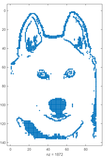
spy
I recently wrote about the new ODE solution framework in MATLAB over the The MATLAB Blog The new solution framework for Ordinary Differential Equations (ODEs) in MATLAB R2023b » The MATLAB Blog - MATLAB & Simulink (mathworks.com)
This was a very popular post at the time - many thousands of views. Clearly everyone cares about ODEs in MATLAB.
This made me wonder. If you could wave a magic wand, what ODE functionality would you have next and why?
Over at Reddit, a MATLAB user asked about when to use a script vs. a live script. How would you answer this?
Starting with MATLAB can be daunting, but the right resources make all the difference. In my experience, the combination of MATLAB Onramp and Cody offers an engaging start.
MATLAB Onramp introduces you to MATLAB's basic features and workflows. Then practice your coding skill on Cody. Challenge yourself to solve 1 basic problem every day for a month! This consistent practice can significantly enhance your proficiency.
What other resources have helped you on your MATLAB journey? Share your recommendations and let's create a comprehensive learning path for beginners!

I'm having problem in its test 6 ... passing 5/6 what would be the real issue..
am wring Transformation matrix correct.. as question said SSW should be 202.5 degree...
so what is the issue..
I would tell myself to understand vectorization. MATLAB is designed for operating on whole arrays and matrices at once. This is often more efficient than using loops.
Is there a reason for TMW not to invest in 3D polyshapes? Is the mathematical complexity of having all the same operations in 3D (union, intersection, subtract,...) prohibitive?
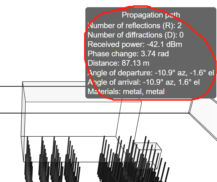
how can I do to get those informations?
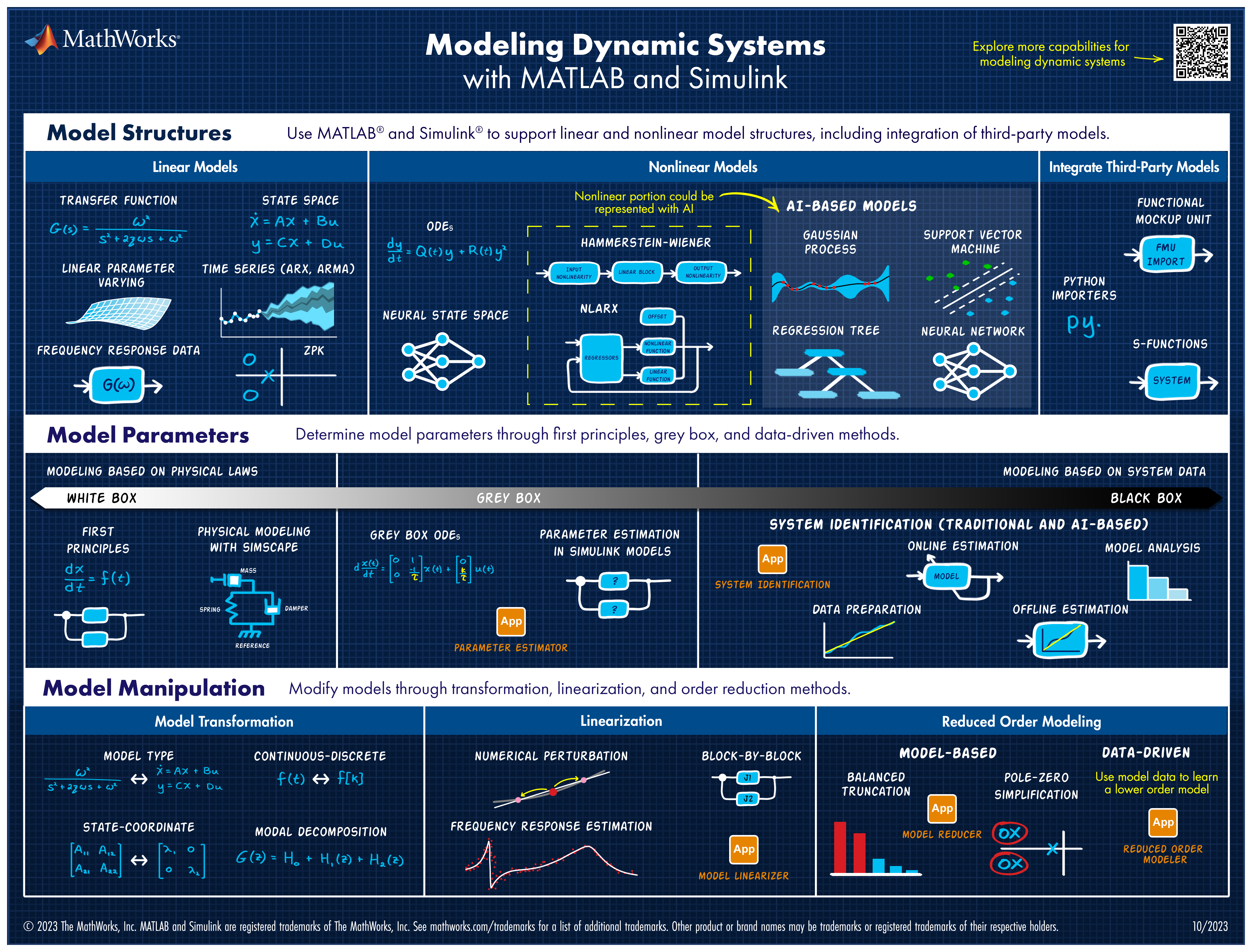
Explore all the capabilities for Modeling Dynamic Systems while keeping them handy with this Cheat Sheet - Download Now.
Quick answer: Add set(hS,'Color',[0 0.4470 0.7410]) to code line 329 (R2023b).
Explanation: Function corrplot uses functions plotmatrix and lsline. In lsline get(hh(k),'Color') is called in for cycle for each line and scatter object in axes. Inside the corrplot it is also called for all axes, which is slow. However, when you first set the color to any given value, internal optimization makes it much faster. I chose [0 0.4470 0.7410], because it is a default color for plotmatrix and corrplot and this setting doesn't change a behavior of corrplot.
Suggestion for a better solution: Add the line of code set(hS,'Color',[0 0.4470 0.7410]) to the function plotmatrix. This will make not only corrplot faster, but also any other possible combinations of plotmatrix and get functions called like this:
h = plotmatrix(A);
% set(h,'Color',[0 0.4470 0.7410])
for k = 1:length(h(:))
get(h(k),'Color');
end
Hello, all!
This is my first post after just joining this discussion, so please forgive me and provide kind assistance if I have posted to the wrong subsection!
I have a good interest in learning sql server course and right now I am taking help from various platforms like https://www.coursera.org/ https://www.udemy.com/
Also I have a doubt that is it a good option to learn from platforms like this or I should go for some sql server online training . I have searched for the solution of my queries in various above platforms which helped me up to some extent only as it was not directly given by any expert or trainer.
Hoping in getting a quick response
Thankyou in advance.
I think it would be a really great feature to be able to add an Alpha property to the basic "Line" class in MATLAB plots. I know that I have previously had to resort to using Patch to be able to plot semitransparent lines, but there are also so many other functions that rely on the "Line" class.
For example, if you want to make a scatter plot from a table with things specified into groups, you can use ScatterHistogram or gscatter but since gscatter uses the Line class, you can't adjust the marker transparency. So if you don't want the histograms, you are stuck with manually separating it and using scatter with hold on.
Hi Guys
Posting this based on a thought I had, so I don't really ahve any code however I would like to know if the thought process is correct and/or relatively accurate.
Consider a simple spring mass system which only allows compression on the spring however when there is tension the mass should move without the effect of the spring distrupting it, thus the mass is just thrown vertically upwards.
The idea which I came up with for such a system is to have two sets of dfferential equations, one which represents the spring system and another which presents a mass in motion without the effects of the spring.
Please refer to the below basic outline of the code which I am proposing. I believe that this may produce relatively decent results. The code essentially checks if there is tension in the system if there is it then takes the last values from the spring mass differential equation and uses it as initial conditions for the differential equation with the mass moving wothout the effects of the spring, this process works in reverse also. The error which would exist is that the initial conditions applied to the system would include effects of the spring. Would there be a better way to code such behaviour?
function xp = statespace(t,x,f,c,k,m)
if (k*x(1)) positive #implying tension
**Use last time step as initial conditions**
**differential equation of a mass moving""
end
if x(1) negative #implying that the mass in now moving down therefore compression in spring
**Use last time step as initial conditions**
**differential equation for a spring mass system**
end
end
Seeing a colleague make this mistake (one I've had to fix multiple times in other's work too) makes me want to ask the community: would you like the awgn() function/blocks to give the option for creating a SNR at the bandwidth of the signal? Your typical flow is something like this:
- Create a signal, usually at some nominal upsampling factor (e.g., 4) such that it's now nicely over sampled, especially if you're using a RRC or similar pulse shaping filter.
- Potentially add a frequency offset (which might make the sample frequency even higher)
- Add AWGN channel model for a desired SNR
- Put this into your detector/receiver model
The problem is, when someone says, "I'm detecting XYZ at foo SNR," it should not magically improve as a function of the oversample. The problem isn't that awgn() generates white noise, that's what it's supposed to do and the typical receiver has noise across the entire band. The problem is that SNR is most properly defined as the signal power over the noise power spectral density times the signal's noise equivalent bandwidth. Now I looked and there's no handy function for computing NEBW for an input signal (there's just a function for assessing analysis windows). In practice it can get a bit tricky. The occupied bandwidth or HPBW are often close enough to the NEBW, we're usually not haggling over hundredths of a dB. So, in my not so humble opinion, the "measured" flag for awgn() should give an option for bandwidth matching or at least document the behavior better in the help page. All too often I'm seeing 3-6 (or worse) dB errors because people aren't taking the signal's bandwidth into account.
Here's a MATLAB class I wrote that leverages the MATLAB Central Interface for MATLAB toolbox, which in turn uses the publicy available Community API. Using this class, I've created a few Favorites that show me what's going on in MATLAB Central - without having to leave MATLAB 🙂
The class has a few convenient queries:
- Results for the last 7 days
- Results for the last 30 days
- Results for the current month
- Results for today
And supporting a bunch of different content scopes:
- All MATLAB Central
- MATLAB Answers
- Blogs
- Cody
- Contests
- File Exchange
- Exclude Answers content
The results are displayed in the command window (which worked best for me) and link to each post. Here's what that looks like for this command
>> CommunityFeed.thisMonth("app designer", CommunityFeed.Scope.ExcludeAnswers)

Let me know if you find this class useful and feel free to suggest changes.
