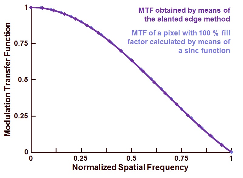
FFT with normalized spatial frequency for image sensor MTF
Ältere Kommentare anzeigen
I'm attempting to use the slanted edge method to calculate the MTF for a camera system according to Harvest Imaging (https://harvestimaging.com/blog/?p=1328), and struggling to plot the result correctly. The method involves taking the Fourier transform of a line spread function and plotting it from DC to the sampling frequency. I have chosen the sampling frequency to equal 2, since that is the minimum number of pixels required to record contrast. Here is my code:
LSF = [];
LSF(1:250) = 0;
LSF(51:70) = 140;
Fs = 2; % Sampling frequency (pixels/lp)
T = 1/Fs; % Sampling period (lp/pixel)
L = length(LSF); % Length of signal (length of line in pixels)
P2 = abs(fft(LSF/L));
P1 = P2(1:L/2+1);
P1(2:end-1) = 2*P1(2:end-1);
f = Fs*(0:(L/2))/L;
nP1 = P1-min(P1);
nP1 = nP1./max(nP1);
plot(f,nP1,'linewidth',3)
title('MTF')
xlabel('Normalized Spatial Frequency')
According to the example, I should reach my first minimum of the sinc function at x=1

But, I appear to be off by a factor of 10.

Can anyone point out where I'm going wrong? I'm sure it's a simple fix.
Thanks much!
7 Kommentare
David Goodmanson
am 20 Apr. 2020
Bearbeitet: David Goodmanson
am 21 Apr. 2020
Hello Ben,
No comment on the interpretation, but a width-two pulse is the only one whose fft is a sinc-like function with its first zero at the edges of the resulting frequency array.
Ben Hendrickson
am 20 Apr. 2020
David Goodmanson
am 21 Apr. 2020
Hello Ben,
I could have been clearer in the comment so I modified it.
Ben Hendrickson
am 21 Apr. 2020
David Goodmanson
am 21 Apr. 2020
Bearbeitet: David Goodmanson
am 21 Apr. 2020
Hello Ben, see these two for a clearer explanation of the method.
The Harvest blog calls the original function (before taking a derivative) the 'spectral frequency response' which I think is confusing if not incorrect. Certainly the idea is to fourier transform a 1d point spread function in pixels to obtain the modulation transfer function in cycles / pixel. Knowing pixel pitch produces cycles per mm. Then a factor of 1/2 to get line pairs / mm ?
Ben Hendrickson
am 21 Apr. 2020
Ali Madani
am 22 Okt. 2020
Hi Ben, did you figure out how to normalized the x-axis? I've been having the same question and cannot figure out how to do this.
Antworten (1)
Hi Ben,
You are off by a factor of 10 because there are 10 samples in one of your 'pixels'. The result of the FT is in cycles/set, which can also be expressed in other units as shown below (see here for a detailed explanation). I used similar figures to yours that however result in the sinc having samples at MTF nulls.
Jack
n = 256; %samples per set
px = 16; %samples per pixel
LSF = zeros(1,n);
LSF(1:px)=140; %the pixel has intensity 140
MTF = 1/sum(LSF) * abs(fft(LSF));
f = 0:n-1; %cycles per set
figure; plot(f,MTF); %cycles per set
xlabel('cycles/set'); ylabel('MTF')
figure; plot(f/n,MTF); %cycles per sample
xlabel('cycles/sample'); ylabel('MTF')
figure; plot (f/n*px,MTF) %cycles per pixel
xlabel('cycles/pixel'); ylabel('MTF'); xlim([0 1])
Kategorien
Mehr zu Fourier Analysis and Filtering finden Sie in Hilfe-Center und File Exchange
Produkte
Community Treasure Hunt
Find the treasures in MATLAB Central and discover how the community can help you!
Start Hunting!
