1-D Decimated Wavelet Transforms
This section takes you through the features of 1-D critically-sampled wavelet analysis using the Wavelet Toolbox™ software.
The toolbox provides these functions for 1-D signal analysis. For more information, see the reference pages.
Analysis-Decomposition Functions
Synthesis-Reconstruction Functions
Decomposition Structure Utilities
Denoising and Compression
Function Name | Purpose |
|---|---|
Automatic wavelet signal denoising (recommended) | |
Penalized threshold for wavelet 1-D or 2-D denoising | |
Thresholds for wavelet 1-D using Birgé-Massart strategy | |
Wavelet denoising and compression | |
Threshold settings manager |
Apps
App | Purpose |
|---|---|
| Signal Multiresolution Analyzer | Decompose signals into time-aligned components |
| Wavelet Signal Analyzer | Analyze and compress signals using wavelets |
| Wavelet Signal Denoiser | Visualize and denoise time series data |
1-D Decimated Wavelet Analysis
This example involves a real-world signal — electrical consumption measured over the course of three days. This signal is particularly interesting because of noise introduced when a defect developed in the monitoring equipment as the measurements were being made. Wavelet analysis effectively removes the noise.
Decomposition and Reconstruction
Load the signal and select a portion for wavelet analysis.
load leleccum
s = leleccum(1:3920);
l_s = length(s);
Use the dwt function to perform a single-level decomposition of the signal using the db1 wavelet. This generates the coefficients of the level 1 approximation (cA1) and detail (cD1).
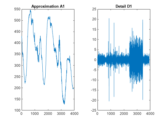
[cA1,cD1] = dwt(s,"db1");Construct the level 1 approximation and detail (A1 and D1) from the coefficients cA1 and cD1. You can use either the idwt function or the upcoef function.
useIDWT =true; if useIDWT A1 = idwt(cA1,[],"db1",l_s); D1 = idwt([],cD1,"db1",l_s); else A1 = upcoef("a",cA1,"db1",1,l_s); D1 = upcoef("d",cD1,"db1",1,l_s); end
Display the results of the level-one decomposition.
tiledlayout(1,2)
nexttile
plot(A1)
title("Approximation A1")
nexttile
plot(D1)
title("Detail D1")
Reconstruct a signal by using the idwt function. Compare the reconstruction with the original signal.
A0 = idwt(cA1,cD1,"db1",l_s);
err = max(abs(s-A0))
err = 2.2737e-13
Use the wavedec function to perform a level 3 decomposition of the signal.
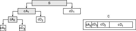
[C,L] = wavedec(s,3,"db1");The coefficients of all the components of a third-level decomposition (that is, the third-level approximation and the first three levels of detail) are returned concatenated into one vector, C. Vector L gives the lengths of each component.
Use the appcoef function to extract the level 3 approximation coefficients from C.
cA3 = appcoef(C,L,"db1",3);Use the detcoef function to extract the levels 3, 2, and 1 detail coefficients from C. The detcoef function gives you the option to extract the coefficients at the different levels one at a time.
extractTogether =true; if extractTogether [cD1,cD2,cD3] = detcoef(C,L,[1,2,3]); else cD3 = detcoef(C,L,3); cD2 = detcoef(C,L,2); cD1 = detcoef(C,L,1); end
Use the wrcoef function to reconstruct the Level 3 approximation and the Level 1, 2, and 3 details.
A3 = wrcoef("a",C,L,"db1",3);
Reconstruct the details at levels 1, 2, and 3.
D1 = wrcoef("d",C,L,"db1",1);
D2 = wrcoef("d",C,L,"db1",2);
D3 = wrcoef("d",C,L,"db1",3);
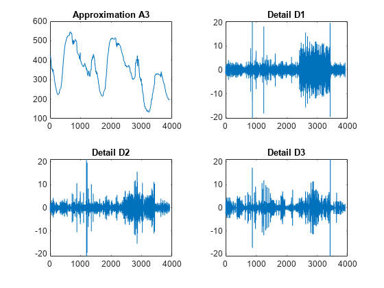
Display the results of the level 3 decomposition.
figure
tiledlayout(2,2)
nexttile
plot(A3)
title("Approximation A3")
nexttile
plot(D1)
title("Detail D1")
nexttile
plot(D2)
title("Detail D2")
nexttile
plot(D3)
title("Detail D3")
Reconstruct the original signal from the Level 3 decomposition.
A0 = waverec(C,L,"db1");
err = max(abs(s-A0))
err = 4.5475e-13
Crude Denoising
Using wavelets to remove noise from a signal requires identifying which component or components contain the noise, and then reconstructing the signal without those components.
In this example, we note that successive approximations become less and less noisy as more and more high-frequency information is filtered out of the signal. The level 3 approximation, A3, is quite clean as a comparison between it and the original signal.
Compare the approximation to the original signal.
figure
tiledlayout(2,1)
nexttile
plot(s)
title("Original")
axis off
nexttile
plot(A3)
title("Level 3 Approximation")
axis off
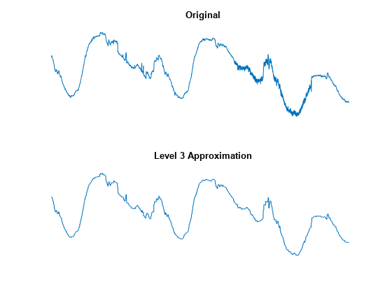
Of course, in discarding all the high-frequency information, we've also lost many of the original signal's sharpest features.
Optimal denoising requires a more subtle approach called thresholding. This involves discarding only the portion of the details that exceeds a certain limit.
Denoise by Thresholding
Let's look again at the details of our level 3 analysis. Display the details D1, D2, and D3.
figure
tiledlayout(3,1)
nexttile
plot(D1)
title("Detail Level 1")
axis off
nexttile
plot(D2)
title("Detail Level 2")
axis off
nexttile
plot(D3)
title("Detail Level 3")
axis off
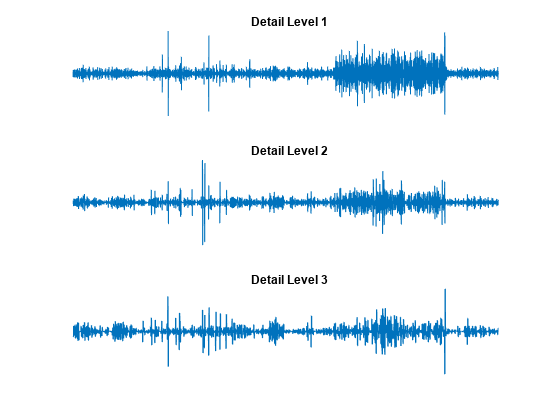
Most of the noise occurs in the latter part of the signal, where the details show their greatest activity. What if we limited the strength of the details by restricting their maximum values? This would have the effect of cutting back the noise while leaving the details unaffected through most of their durations. But there's a better way.
Note that cD1, cD2, and cD3 are vectors, so we could directly manipulate each vector, setting each element to some fraction of the vectors' peak or average value. Then we could reconstruct new detail signals D1, D2, and D3 from the thresholded coefficients.
To denoise a signal, use the wdenoise function. The wdenoise function is recommended for denoising 1-D signals. The function provides a simple interface to a variety of denoising methods. Default parameters are provided are automatically provided for quick and easy use.
Instead of using all the default function values, denoise the signal using the db1 wavelet and a wavelet decomposition down to level 3.
clean = wdenoise(s,3,Wavelet="db1");Display the original and denoised signals. Notice how we have removed the noise without compromising the sharp detail of the original signal. This is a strength of wavelet analysis.
figure
tiledlayout(2,1)
nexttile
plot(s(2000:3920))
title("Original")
nexttile
plot(clean(2000:3920))
title("Denoised")
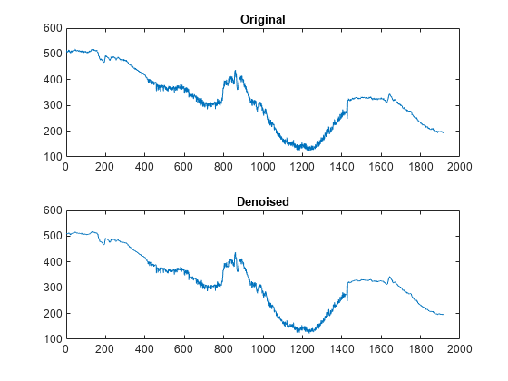
We have plotted here only the noisy latter part of the signal. Notice how we have removed the noise without compromising the sharp detail of the original signal. This is a strength of wavelet analysis.
You can also use the Wavelet Signal Denoiser app to denoise 1-D signals.