Main Content

scatteringTransform

Wavelet 2-D scattering transform

Description

s = scatteringTransform(sf,im) returns the wavelet 2-D scattering transform of im for sf, the image scattering network. im is a real-valued 2-D matrix or 3-D matrix. If im is 3-D, the size of the third dimension must equal 3. The row and column sizes of im must match the ImageSize value of sf. The output s is a cell array with Nfb+1 elements, where Nfb is the number of filter banks in the scattering network. Nfb is equal to the number of elements in the QualityFactors property of sf. Equivalently, the number of elements in s is equal to the number of orders in the scattering network. Each element of s is a MATLAB® table.

example

[s,u] = scatteringTransform(sf,im) also returns the wavelet scalogram coefficients for im. The output u is a cell array with Nfb+1 elements, where Nfb is the number of filter banks in the scattering network. Nfb is equal to the number of elements in the QualityFactors property of sf. Equivalently, the number of elements in u is equal to the number of orders in the scattering network. Each element of u is a MATLAB table.

Examples

collapse all

This example shows that scattering coefficients are lowpassed versions of scalogram coefficients.

Load an RGB image. Display the red channel.

im = imread('circle.jpg');
size(im)
ans = 1×3

   256   256     3

figure
imagesc(im(:,:,1))
colormap gray;

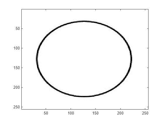
For RGB images, the size of the third dimension must be 3. You only have to specify the row and column sizes of the image when you create the scattering network. Create a scattering network to apply to the image and take the scattering transform.

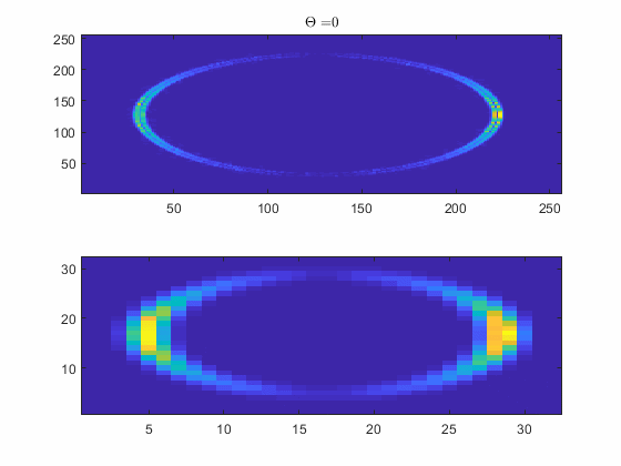
sf = waveletScattering2('ImageSize',[256 256],'InvarianceScale',32,...
    'NumRotations',[8 8]);
[S,U] = scatteringTransform(sf,im);

The image and coefficient fields in S and U are M-by-N-by-3. The M-by-N dimensions are constant only in the scattering images because the scaling function has fixed bandwidth, while the wavelets have different bandwidths.

Use a for-loop and plot the red channel for the scalogram and scattering coefficients for the 8 rotation angles in the scattering transform. Note how the scattering coefficients are lowpass versions of the scalogram coefficients.

[~,~,~,filterparams] = sf.filterbank();
theta = filterparams{1}.rotations;
figure
for k = 1:numel(theta)
    subplot(2,1,1)
    imagesc(U{2}.coefficients{k}(:,:,1));
    axis xy
    title(['$$\Theta =  $$' num2str(theta(k))],'Interpreter','Latex');
    subplot(2,1,2)
    imagesc(S{2}.images{k}(:,:,1)); 
    axis xy
    pause(1)
end

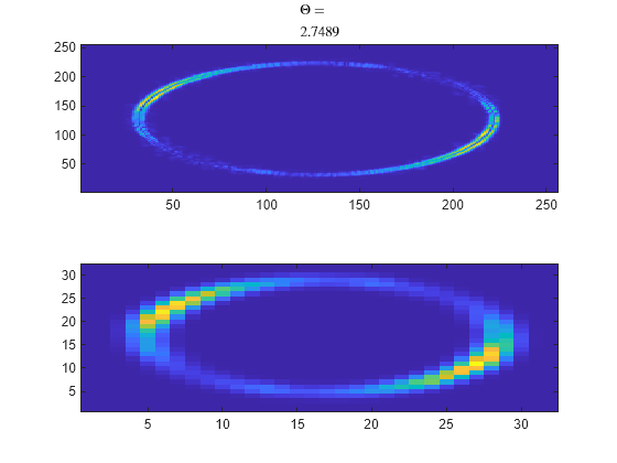
The above for-loop results in an animation identical to the one below.

Input Arguments

collapse all

Wavelet image scattering network, specified as a waveletScattering2 object.

Input image, specified as a real-valued 2-D matrix or 3-D matrix. If im is 3-D, im is assumed to be a color image in the RGB color space, and the size of the third dimension must equal 3. The row and column sizes of im must match the ImageSize property of sf.

Output Arguments

collapse all

Scattering coefficients, returned as a cell array. s is a cell array with Nfb+1 elements where Nfb is the number of filter banks in the scattering network. Nfb is equal to the number of elements in the QualityFactors property of sf. Equivalently, the number of elements in s is equal to the number of orders in the scattering network. Each element of s is a MATLAB table with these variables:

Scattering coefficients, returned as a cell array. Each element of images is an M-by-N or M-by-N-by-3 matrix.

Scattering path used to obtain the scattering coefficients, returned as a row vector. Each column of path corresponds to one element of the path. The scalar 0 denotes the original image. Positive integers in the Lth column denote the corresponding wavelet filter in the (L−1)th filter bank. Wavelet bandpass filters are ordered by decreasing center frequency.

There are NumRotations wavelets per center frequency pair.

Bandwidth of scattering coefficients, returned as a scalar. The bandwidth is symmetric in the x and y directions.

Base-2 log resolution of the scattering coefficients, returned as a scalar.

Scalogram coefficients, returned as a cell array. u is a cell array with Nfb+1 elements, where Nfb is the number of filter banks in the scattering network. Nfb is equal to the number of elements in the QualityFactors property of sf. Equivalently, the number of elements in u is equal to the number of orders in the scattering network. Each element of u is a MATLAB table with these variables:

Scalogram coefficients, returned as a cell array. Each element of coefficients is an M-by-N or M-by-N-by-3 matrix.

Scattering path used to obtain the scalogram coefficients, returned as a row vector. Each column of path corresponds to one element of the path. The scalar 0 denotes the original image. Positive integers in the Lth column denote the corresponding wavelet filter in the (L−1)th filter bank. Wavelet bandpass filters are ordered by decreasing center frequency.

There are NumRotations wavelets per center frequency pair.

Bandwidth of scalogram coefficients, returned as a scalar.

Base-2 log resolution of the scattering coefficients, returned as a scalar.

Version History

Introduced in R2019a