Main Content

ilwt2

Inverse 2-D lifting wavelet transform

Since R2021b

    Description

    xr = ilwt2(ll,lh,hl,hh) returns the 2-D inverse wavelet transform based on the approximation coefficients, ll, and the horizontal (lh), vertical (hl), and diagonal (hh) wavelet coefficients. By default, ilwt2 assumes that you used the lifting scheme associated with the db1 wavelet to obtain the coefficients. If you have not modified the coefficients, xr is a perfect reconstruction of the signal.

    example

    xr = ilwt2(ll,lh,hl,hh,Name=Value) specifies options using one or more name-value arguments. For example, ilwt2(ll,lh,hl,hh,LiftingScheme=lscheme,Level=3) specifies the lscheme lifting scheme and the inverse transform up to level 3.

    example

    Examples

    collapse all

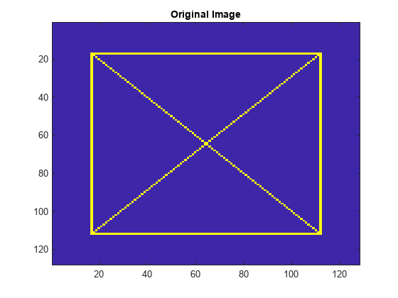
    Load and display the 128-by-128 xbox image.

    load xbox
    imagesc(xbox)
    title("Original Image")

    Figure contains an axes object. The axes object with title Original Image contains an object of type image.

    Obtain the 2-D LWT of the image using default settings. Preserve integer values.

    [ll,lh,hl,hh] = lwt2(xbox,Int2Int=true);

    Obtain the inverse LWT up to level 1. Confirm the size of the reconstruction is 64-by-64.

    xr = ilwt2(ll,lh,hl,hh,Level=1,Int2Int=true);
    size(xr)
    ans = 1×2
    
        64    64
    
    
    imagesc(xr)
    title("Level 1 Reconstruction")

    Figure contains an axes object. The axes object with title Level 1 Reconstruction contains an object of type image.

    Obtain the inverse LWT using default settings. Confirm perfect reconstruction.

    xr = ilwt2(ll,lh,hl,hh,Int2Int=true);
    max(abs(xr(:)-xbox(:)))
    ans = 
    0
    

    Load the 3-D wmri data set. The data consists of 27 128-by-128 magnetic resonance images (MRI) arranged in a 128-by-128-by-27 array.

    load wmri

    Display some of the slices along the Z-orientation of the original data set.

    map = pink(90);
    idxImages = 1:3:size(X,3);
    figure("DefaultAxesXTick",[],"DefaultAxesYTick",[],...
        "DefaultAxesFontSize",8,"Color","w")
    colormap(map)
    for k = 1:9
        j = idxImages(k);
        subplot(3,3,k)
        image(X(:,:,j))
        str = sprintf("Z = %d",j);
        title(str)
    end

    Figure contains 9 axes objects. Axes object 1 with title Z = 1 contains an object of type image. Axes object 2 with title Z = 4 contains an object of type image. Axes object 3 with title Z = 7 contains an object of type image. Axes object 4 with title Z = 10 contains an object of type image. Axes object 5 with title Z = 13 contains an object of type image. Axes object 6 with title Z = 16 contains an object of type image. Axes object 7 with title Z = 19 contains an object of type image. Axes object 8 with title Z = 22 contains an object of type image. Axes object 9 with title Z = 25 contains an object of type image.

    By default, lwt2 performs the wavelet decomposition along the rows and columns of the input data. Use lwt2 to obtain the 2-D LWT of each 128-by-128 slice in the 3-D data set using the lifting scheme associated with the bior3.5 wavelet. Preserve the integer-valued data.

    lscheme = liftingScheme(Wavelet="bior3.5");
    [ll,lh,hl,hh] = lwt2(X,LiftingScheme=lscheme,Int2Int=true);

    Inspect the dimensions of a detail coefficients cell array. Confirm the coefficients at each level is a 3-D array, and the size of the third dimension is 27.

    hh
    hh=7×1 cell array
        {64x64x27 double}
        {32x32x27 double}
        {16x16x27 double}
        { 8x8x27  double}
        { 4x4x27  double}
        { 2x2x27  double}
        { 1x1x27  double}


    Obtain the inverse 2-D LWT up to level 1. Confirm the size of the 3-D reconstruction is 64-by-64-by-27.

    xr = ilwt2(ll,lh,hl,hh,LiftingScheme=lscheme,Int2Int=true,Level=1);
    size(xr)
    ans = 1×3
    
        64    64    27


    Choose any slice from the original data set, and perform the same LWT operations on that slice. Confirm the reconstruction is equal to the corresponding slice in the 3-D reconstruction array.

    num = 13;
    slice = X(:,:,num);
    [lls,lhs,hls,hhs] = lwt2(slice,LiftingScheme=lscheme,Int2Int=true);
    xrs = ilwt2(lls,lhs,hls,hhs,LiftingScheme=lscheme,Int2Int=true,Level=1);
    max(max(abs(xrs-xr(:,:,num))))
    ans = 
    0
    

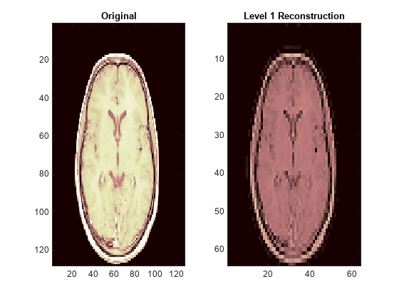
    Compare the reconstruction of the slice with the original version.

    figure
    colormap(map)
    subplot(1,2,1)
    image(X(:,:,num))
    title("Original")
    subplot(1,2,2)
    image(xrs)
    title("Level 1 Reconstruction")

    Figure contains 2 axes objects. Axes object 1 with title Original contains an object of type image. Axes object 2 with title Level 1 Reconstruction contains an object of type image.

    Input Arguments

    collapse all

    Approximation coefficients at the coarsest scale, specified as a scalar, vector, or matrix. The coefficients are the output of lwt2.

    Data Types: single | double
    Complex Number Support: Yes

    Horizontal detail coefficients by level, specified as a LEV-by-1 cell array, where LEV is the level of the decomposition. The elements of lh are in order of decreasing resolution. The coefficients are the output of lwt2.

    Data Types: single | double
    Complex Number Support: Yes

    Vertical detail coefficients by level, specified as a LEV-by-1 cell array, where LEV is the level of the decomposition. The elements of hl are in order of decreasing resolution. The coefficients are the output of lwt2.

    Data Types: single | double
    Complex Number Support: Yes

    Diagonal detail coefficients by level, specified as a LEV-by-1 cell array, where LEV is the level of the decomposition. The elements of hh are in order of decreasing resolution. The coefficients are the output of lwt2.

    Data Types: single | double
    Complex Number Support: Yes

    Name-Value Arguments

    Specify optional pairs of arguments as Name1=Value1,...,NameN=ValueN, where Name is the argument name and Value is the corresponding value. Name-value arguments must appear after other arguments, but the order of the pairs does not matter.

    Example: xr = ilwt2(ll,lh,hl,hh,Wavelet="db2",Int2Int=true)

    Orthogonal or biorthogonal wavelet to use in the inverse LWT, specified as a character vector or string scalar. See the Wavelet property of liftingScheme for the list of supported wavelets. For perfect reconstruction, you must specify the same wavelet that you used to obtain the coefficients ll, lh, hl, and hh.

    You cannot specify Wavelet and LiftingScheme at the same time.

    Example: xr = ilwt2(ll,lh,hl,hh,Wavelet="bior3.5") uses the bior3.5 biorthogonal wavelet.

    Data Types: char | string

    Lifting scheme to use in the inverse LWT, specified as a liftingScheme object. For perfect reconstruction, you must specify the same lifting scheme that you used to obtain the coefficients ll, lh, hl, and hh.

    You cannot specify LiftingScheme and Wavelet at the same time.

    Example: xr = ilwt2(ll,lh,hl,hh,LiftingScheme=lScheme) uses the lScheme lifting scheme.

    Reconstruction level, specified as a nonnegative integer less than or equal to length(hh)-1. If you do not specify a level, the function sets the reconstruction level to 0 and xr is a perfect reconstruction of the signal.

    Example: xr = ilwt2(ll,lh,hl,hh,Level=2) reconstructs the signal up to level 2.

    Data Types: double

    Extension mode to use in the inverse LWT, specified as one of these:

    • "periodic" — Periodized extension

    • "zeropad" — Zero extension

    • "symmetric" — Symmetric extension

    This argument specifies how to extend the signal at the boundaries.

    Example: xr = ilwt2(ll,lh,hl,hh,Extension="zeropad") specifies zero extension.

    Integer-valued data handling, specified as one of these:

    • 1 (true) — Preserve integer-valued data

    • 0 (false) — Do not preserve integer-valued data

    Specify Int2Int only if all coefficients are integers.

    Example: xr = ilwt2(ll,lh,hl,hh,Int2Int=true) preserves integer-valued data.

    Output Arguments

    collapse all

    Inverse wavelet transform, returned as a matrix. xr has the same dimensionality as the input used by the lwt2 function to generate the approximation and details coefficients.

    References

    [1] Strang, Gilbert, and Truong Nguyen. Wavelets and Filter Banks. Rev. ed. Wellesley, Mass: Wellesley-Cambridge Press, 1997.

    [2] Sweldens, Wim. “The Lifting Scheme: A Construction of Second Generation Wavelets.” SIAM Journal on Mathematical Analysis 29, no. 2 (March 1998): 511–46. https://doi.org/10.1137/S0036141095289051.

    Extended Capabilities

    C/C++ Code Generation
    Generate C and C++ code using MATLAB® Coder™.

    Version History

    Introduced in R2021b

    expand all

    Go to top of page