dldwt

Differentiable discrete wavelet transform

Since R2025a

Syntax

[A,D] = dldwt(X)

[A,D] = dldwt(X,Name=Value)

Description

[A,D] = dldwt(X) returns the approximation coefficients A and wavelet coefficients D of the deep learning discrete wavelet transform (DWT) of X. By default, dldwt obtains the DWT at level 1 using the Haar wavelet and "reflection" padding at the boundary.

[A,D] = dldwt(X,Name=Value) specifies options using one or more name-value arguments. For example, PaddingMode="zeropad" specifies zero padding at the boundary.

Examples

Deep Learning Discrete Wavelet Transform

1-D DWT

Load the wecg signal. The data is arranged as a 2048-by-1 vector.

load wecg

Create a formatted dlarray object that represents the signal to use with the dldwt function. Specify the format "TCB", so that the time dimension corresponds to the column dimension and the channel dimension corresponds to the row dimension. Note that, in this case, specifying "TBC" will also work because in both cases, the dlarray function will permute the dimensions of the signal to 1-by-1-by-2048.

wecgdl = dlarray(wecg,"TCB");

Use the dldwt function with default values to obtain the deep learning DWT of the signal. The result is the single-level DWT of the signal using the Haar wavelet. Inspect the dimensions of the approximation and wavelet coefficients. Confirm both tensors are dlarray objects in "CBT" format.

[aTime,dTime] = dldwt(wecgdl);
size(aTime)

ans = 1×3

           1           1        1024

size(dTime)

ans = 1×3

           1           1        1024

dims(aTime)

ans = 
'CBT'

dims(dTime)

ans = 
'CBT'

Create an array that contains two copies of the wecg signal along the second dimension.

wecg2 = repmat(wecg,1,2);
size(wecg2)

ans = 1×2

        2048           2

Create a formatted dlarray that represents the new array. As before, the column dimension corresponds to time. However, unlike the case of the original signal, how dlarray will permute the data depends on whether the second dimension corresponds to the channel dimension or batch dimension. Specify the format "TCB". Obtain the DWT and inspect the sizes of the output coefficients.

wecg2dl = dlarray(wecg2,"TCB");
[aTime2a,dTime2a] = dldwt(wecg2dl);
size(aTime2a)

ans = 1×3

           2           1        1024

size(dTime2a)

ans = 1×3

           2           1        1024

Now create a dlarray with format "TBC" and obtain the DWT. Confirm the sizes of the coefficients are different.

wecg2dl = dlarray(wecg2,"TBC");
[aTime2b,dTime2b] = dldwt(wecg2dl);
size(aTime2b)

ans = 1×3

           1           2        1024

size(dTime2b)

ans = 1×3

           1           2        1024

Both sets of coefficients, though, have the same format.

dims(aTime2a)

ans = 
'CBT'

dims(aTime2b)

ans = 
'CBT'

dims(dTime2a)

ans = 
'CBT'

dims(dTime2b)

ans = 
'CBT'

2-D DWT

Load the xbox image. The image is arranged as a 128-by-128 matrix.

load xbox

Cast the image to single precision. Create a dlarray object that represents the image. Specify the format "SSCB". The spatial dimensions correspond to the height and width of the image.

load xbox
xboxs = single(xbox);
xboxsdl = dlarray(xboxs,"SSCB");

Obtain the deep learning DWT of the image. Inspect the dimensions of the approximation and wavelet coefficients. Confirm both tensors are dlarray objects.

[aImage,dImage] = dldwt(xboxsdl);
size(aImage)

ans = 1×4

    64    64     1     1

size(dImage)

ans = 1×4

    64    64     3     1

dims(aImage)

ans = 
'SSCB'

dims(dImage)

ans = 
'SSCB'

Confirm the underlying data type of both tensors is single.

underlyingType(aImage)

ans = 
'single'

underlyingType(dImage)

ans = 
'single'

Full Deep Learning Wavelet Decomposition of Signal

Load the wecg signal. Cast the signal to single precision and save as a gpuArray object.

load wecg
sig = gpuArray(single(wecg));

Use dldwt to obtain the DWT of the signal down to level 5. Obtain the wavelet coefficients at all levels. Specify the db4 wavelet and periodic boundary handling. Because the input is a numeric array, you must specify the data format. Set DataFormat to "TCB". The function returns the approximation coefficients, a, and wavelet coefficients, d, as unformatted dlarray objects.

wv = "db4";
lv = 5;
[a,d] = dldwt(sig,Wavelet=wv,Level=lv, ...
    FullTree=true, ...
    PaddingMode="periodic", ...
    DataFormat="TCB");

Inspect the approximation coefficients. Extract the approximation coefficients and confirm they are a gpuArray with underlying data type single.

appcfs = extractdata(a);
isgpuarray(appcfs)

ans = logical
   1

underlyingType(appcfs)

ans = 
'single'

Inspect the wavelet coefficients. The function returns the wavelet coefficients in a 5-by-1 cell array. Each element contains the wavelet coefficients at that level.

d

d=5×1 cell array
    {1×1×1024 dlarray}
    {1×1×512  dlarray}
    {1×1×256  dlarray}
    {1×1×128  dlarray}
    {1×1×64   dlarray}

Extract the wavelet coefficients from the cell array. Each element is a gpuArray in single precision.

wavcfs = cellfun(@(x)extractdata(x),d,UniformOutput=false)

wavcfs=5×1 cell array
    {1×1×1024 gpuArray}
    {1×1×512  gpuArray}
    {1×1×256  gpuArray}
    {1×1×128  gpuArray}
    {1×1×64   gpuArray}

cellfun(@(x)underlyingType(x),wavcfs,UniformOutput=false)

ans = 5×1 cell
    {'single'}
    {'single'}
    {'single'}
    {'single'}
    {'single'}

Use wavedec to obtain the DWT of the original signal. Use the same wavelet, decomposition level, and boundary extension mode as before. Then use appcoef and detcoef to obtain the approximation and wavelet coefficients, respectively, from the decomposition.

[c,l] = wavedec(sig,lv,wv,Mode="per");
cApp = appcoef(c,l,wv,mode="per");
cWav = detcoef(c,l,"cells");

Compare the approximation coefficients computed using dldwt and wavedec. Confirm the norm of their differences is virtually zero.

appcfs = reshape(appcfs,[],1);
norm(appcfs-cApp,Inf)

ans =

  gpuArray single

  4.7684e-07

Compare the wavelet coefficients.

cWav = cWav';
tmpcfs = cellfun(@(x)reshape(x,[],1),wavcfs,UniformOutput=false);
cellfun(@(x,y)norm(x-y,Inf),cWav,tmpcfs)

ans =

  5×1 gpuArray single column vector

   1.0e-06 *

    0.0596
    0.3576
    0.4768
    0.3427
    0.3576

Discrete Wavelet Transform of 2-D Multichannel Image

Load the xbox and tartan images. Each image is a 128-by-128 matrix.

load xbox
load tartan
tartan = X;
tiledlayout(1,2)
nexttile
imagesc(xbox)
set(gca,'xtick',[])
set(gca,'ytick',[])
title("xbox")
nexttile
imagesc(tartan)
set(gca,'xtick',[])
set(gca,'ytick',[])
title("tartan")

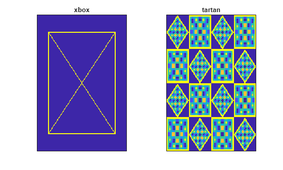
Create a random 2-D multichannel image with five channels. The size of the row and column dimensions are 128. Store the xbox image in the first channel and the tartan image in the fourth channel.

ind1 = 1;
ind2 = 4;
nchan = 5;
img = randn(128,128,nchan);
img(:,:,ind1) = xbox;
img(:,:,ind2) = tartan;

Use dldwt to obtain the DWT of the multichannel image using the bior4.4 wavelet. Because the input is a numeric array, you must specify the data format. Set DataFormat to "SSCB". The function returns the approximation coefficients, a, and wavelet coefficients, d, as unformatted dlarray objects.

[a,d] = dldwt(img,Wavelet="bior4.4",DataFormat="SSCB");

Extract the approximation and wavelet coefficients from the two tensors. Inspect their dimensions. The input data and approximation coefficients array both have the same number of channels. To account for the three different orientations or subbands, LH (horizontal), HL (vertical), and HH (diagonal), the wavelet coefficients array has three times as many channels.

allApprox = extractdata(a);
allDetails = extractdata(d);
size(allApprox)

ans = 1×3

    68    68     5

size(allDetails)

ans = 1×3

    68    68    15

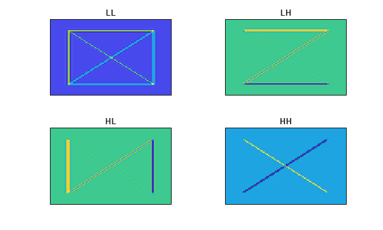
Obtain and plot the approximation and wavelet coefficients of the xbox image.

xboxApprox = allApprox(:,:,ind1);
xboxDetails = allDetails(:,:,ind1+nchan*[0 1 2]);
figure
tiledlayout(2,2)
nexttile
imagesc(xboxApprox)
set(gca,'xtick',[])
set(gca,'ytick',[])
title("LL")
nexttile
imagesc(xboxDetails(:,:,1))
set(gca,'xtick',[])
set(gca,'ytick',[])
title("LH")
nexttile
imagesc(xboxDetails(:,:,2))
set(gca,'xtick',[])
set(gca,'ytick',[])
title("HL")
nexttile
imagesc(xboxDetails(:,:,3))
set(gca,'xtick',[])
set(gca,'ytick',[])
title("HH")

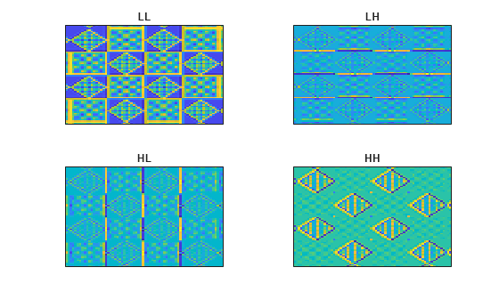
Obtain and plot the approximation and wavelet coefficients of the tartan image.

tartanApprox = allApprox(:,:,ind2);
tartanDetails = allDetails(:,:,ind2+nchan*[0 1 2]);
figure
tiledlayout(2,2)
nexttile
imagesc(tartanApprox)
set(gca,'xtick',[])
set(gca,'ytick',[])
title("LL")
nexttile
imagesc(tartanDetails(:,:,1))
set(gca,'xtick',[])
set(gca,'ytick',[])
title("LH")
nexttile
imagesc(tartanDetails(:,:,2))
set(gca,'xtick',[])
set(gca,'ytick',[])
title("HL")
nexttile
imagesc(tartanDetails(:,:,3))
set(gca,'xtick',[])
set(gca,'ytick',[])
title("HH")

Input Arguments

X — Input data

dlarray object | numeric array

Input data, specified as a real-valued unformatted dlarray object, a formatted dlarray in "CBT" (channel, batch, time) format or "SSCB" (spatial, spatial, channel, batch) format, or a numeric tensor. If X is an unformatted dlarray or a numeric array, you must set DataFormat as one of "CBT" and "SSCB" and X must be compatible with the specified data format.

If X is a dlarray with format "CBT", dldwt computes the 1-D DWT. If X is a dlarray with format "SSCB", dldwt computes the 2-D DWT.

Data Types: single | double

Name-Value Arguments

Specify optional pairs of arguments as Name1=Value1,...,NameN=ValueN, where Name is the argument name and Value is the corresponding value. Name-value arguments must appear after other arguments, but the order of the pairs does not matter.

Example: [A,D] = dldwt(X,Wavelet="db4",Level=5) computes the DWT down to level 5 using the db4 wavelet.

Wavelet — Wavelet

"haar" (default) | character vector | string scalar

Analyzing wavelet, specified as a character vector or string scalar.

dldwt supports only Type 1 (orthogonal) or Type 2 (biorthogonal) wavelets. See wfilters for a list of orthogonal and biorthogonal wavelets.

LowpassFilter,HighpassFilter — Wavelet decomposition filters

numeric vectors | dlarray objects

Wavelet decomposition filters to use in the DWT, specified as a pair of even-length real-valued numeric vectors or unformatted dlarray objects. LowpassFilter is the lowpass (scaling) filter, and HighpassFilter is the highpass (wavelet) filter. For more information, see wfilters.

Example: [A,D] = dldwt(X,LowpassFilter=lf,HighpassFilter=hf)

Level — Decomposition level

1 (default) | positive integer

Decomposition level, specified as a positive integer less than or equal to:

• floor(log2(length(X))), if X is a dlarray in "CBT" format.

• floor(log2(min(size(X,1),size(X,2)))), if X is a dlarray in "SSCB" format.

Data Types: single | double

PaddingMode — DWT extension mode

"reflection" (default) | "periodic" | "zeropad"

DWT extension mode, specified as "reflection" , "periodic", or "zeropad". dldwt extends the coefficients at the boundary at each level based on the corresponding mode in dwtmode:

• "reflection" — Half-point symmetric extension, "sym"

• "periodic" — Periodic extension, "per"

• "zeropad" — Zero padding, "zpd"

FullTree — Full wavelet decomposition option

false or 0 (default) | true or 1

Full wavelet decomposition option, specified as a numeric or logical 1 (true) or 0 (false).

To return the wavelet coefficients at all levels, set FullTree to true. If Level is greater than 1, D is a cell array of tensors. If FullTree is set to false, only the final level (coarsest resolution) wavelet coefficients are returned.

DataFormat — Input data format

character vector | string scalar

Input data format, specified as some permutation of "CBT" or "SSCB". This argument is valid only if X is unformatted. If the input data is a formatted dlarray and you specify DataFormat, the dldwt function will error.

Each character in this argument must be one of these labels:

• S — Spatial

• C — Channel

• B — Batch

• T — Time

The dldwt function accepts any permutation of "CBT" or "SSCB". Each element of the argument labels the matching dimension of X.

The dimension order of dldwt outputs are always "CBT" or "SSCB".

Example: w = dldwt(X,DataFormat="BCT") specifies the data format of the unformatted dlarray object as "BCT".

Data Types: char | string

Output Arguments

A — Approximation coefficients

dlarray object

Approximation coefficients at the final level (coarsest resolution), returned as a dlarray object (tensor).

• If X is a formatted dlarray, then A is a dlarray in "CBT" or "SSCB" format.

• If X is an unformatted dlarray or a numeric array, then A is an unformatted dlarray. The dimension order in A is "CBT" or "SSCB".

For more information, see wavedec and wavedec2.

D — Wavelet coefficients

dlarray object | cell array

Wavelet coefficients at the final level (coarsest resolution), returned as a dlarray object (tensor). If X is a formatted dlarray, then D is a dlarray in "CBT" or "SSCB" format. If X is an unformatted dlarray or a numeric array, then D is an unformatted dlarray. The dimension order in D is "CBT" or "SSCB".

If the size of the "C" (channel) dimension of X is N, the size of the channel dimension of D is:

• N, if X is compatible with format "CBT". For more information, see wavedec.

• 3N, if X is compatible with format "SSCB". The order of the wavelet subbands along the channel dimension is LH (horizontal details), HL (vertical details), and HH (diagonal details), where H denotes highpass filtering and L denotes lowpass filtering.

  To elaborate, the dldwt function replicates each subband for all channels. For example, for a 2-D multichannel image with five channels of size M-by-M-by-5, the one-level DWT is an N-by-N-by-15 array, where the first five pages are all the HL subbands, the next five pages are the LH subbands, and the next five pages are the HH subbands.

  To learn more about the wavelet subbands, see wavedec2.

To obtain the full wavelet transform, set FullTree to true. If Level is greater than 1, the wavelet coefficients are returned by level as a cell array of tensors.

Example: If X

Extended Capabilities

GPU Arrays

Accelerate code by running on a graphics processing unit (GPU) using Parallel Computing Toolbox™.

The dldwt function fully supports GPU arrays. To run the function on a GPU, specify the input data as a gpuArray (Parallel Computing Toolbox). For more information, see Run MATLAB Functions on a GPU (Parallel Computing Toolbox).

Version History

Introduced in R2025a