quantilePredict

Predict response quantile using bag of regression trees

Syntax

YFit = quantilePredict(Mdl,X)

YFit = quantilePredict(Mdl,X,Name,Value)

[YFit,YW] = quantilePredict(___)

Description

YFit = quantilePredict(Mdl,X) returns a vector of medians of the predicted responses at X, a table or matrix of predictor data, and using the bag of regression trees Mdl. Mdl must be a TreeBagger model object.

YFit = quantilePredict(Mdl,X,Name,Value) uses additional options specified by one or more Name,Value pair arguments. For example, specify quantile probabilities or which trees to include for quantile estimation.

[YFit,YW] = quantilePredict(___) also returns a sparse matrix of response weights.

Input Arguments

Mdl — Bag of regression trees

TreeBagger model object (default)

Bag of regression trees, specified as a TreeBagger model object created by the TreeBagger function. The value of Mdl.Method must be regression.

X — Predictor data

numeric matrix | table

Predictor data used to estimate quantiles, specified as a numeric matrix or table.

Each row of X corresponds to one observation, and each column corresponds to one variable.

• For a numeric matrix:

  • The variables making up the columns of X must have the same order as the predictor variables that trained Mdl.

  • If you trained Mdl using a table (for example, Tbl), then X can be a numeric matrix if Tbl contains all numeric predictor variables. If Tbl contains heterogeneous predictor variables (for example, numeric and categorical data types) and X is a numeric matrix, then quantilePredict throws an error.

• For a table:

  • quantilePredict does not support multicolumn variables and cell arrays other than cell arrays of character vectors.

  • If you trained Mdl using a table (for example, Tbl), then all predictor variables in X must have the same variable names and data types as those variables that trained Mdl (stored in Mdl.PredictorNames). However, the column order of X does not need to correspond to the column order of Tbl. Tbl and X can contain additional variables (response variables, observation weights, etc.), but quantilePredict ignores them.

  • If you trained Mdl using a numeric matrix, then the predictor names in Mdl.PredictorNames and corresponding predictor variable names in X must be the same. To specify predictor names during training, see the PredictorNames name-value pair argument of the TreeBagger function. All predictor variables in X must be numeric vectors. X can contain additional variables (response variables, observation weights, etc.), but quantilePredict ignores them.

Data Types: table | double | single

Name-Value Arguments

Specify optional pairs of arguments as Name1=Value1,...,NameN=ValueN, where Name is the argument name and Value is the corresponding value. Name-value arguments must appear after other arguments, but the order of the pairs does not matter.

Before R2021a, use commas to separate each name and value, and enclose Name in quotes.

Quantile — Quantile probability

0.5 (default) | numeric vector containing values in [0,1]

Quantile probability, specified as the comma-separated pair consisting of 'Quantile' and a numeric vector containing values in the interval [0,1]. For each observation (row) in X, quantilePredict returns corresponding quantiles for all probabilities in Quantile.

Example: 'Quantile',[0 0.25 0.5 0.75 1]

Data Types: single | double

Trees — Indices of trees to use in response estimation

'all' (default) | numeric vector of positive integers

Indices of trees to use in response estimation, specified as the comma-separated pair consisting of 'Trees' and 'all' or a numeric vector of positive integers. Indices correspond to the cells of Mdl.Trees; each cell therein contains a tree in the ensemble. The maximum value of Trees must be less than or equal to the number of trees in the ensemble (Mdl.NumTrees).

For 'all', quantilePredict uses the indices 1:Mdl.NumTrees.

Example: 'Trees',[1 10 Mdl.NumTrees]

Data Types: char | string | single | double

TreeWeights — Weights to attribute to responses from individual trees

numeric vector of nonnegative values

Weights to attribute to responses from individual trees, specified as the comma-separated pair consisting of 'TreeWeights' and a numeric vector of numel(trees) nonnegative values. trees is the value of the Trees name-value pair argument.

The default is ones(size(trees)).

Data Types: single | double

UseInstanceForTree — Indicators specifying which trees to use to make predictions for each observation

'all' (default) | logical matrix

Indicators specifying which trees to use to make predictions for each observation, specified as the comma-separated pair consisting of 'UseInstanceForTree' and an n-by-Mdl.Trees logical matrix. n is the number of observations (rows) in X. Rows of UseInstanceForTree correspond to observations and columns correspond to learners in Mdl.Trees. 'all' indicates to use all trees for all observations when estimating the quantiles.

If UseInstanceForTree(j,k) = true, then quantilePredict uses the tree in Mdl.Trees(trees(k)) when it predicts the response for the observation X(j,:).

You can estimate the quantile using the response data in Mdl.Y directly instead of using the predictions from the random forest by specifying a row composed entirely of false values. For example, to estimate the quantile for observation j using the response data, and to use the predictions from the random forest for all other observations, specify this matrix:

UseInstanceForTree = true(size(Mdl.X,2),Mdl.NumTrees);
UseInstanceForTree(j,:) = false(1,Mdl.NumTrees);

Data Types: char | string | logical

Output Arguments

YFit — Estimated quantiles

numeric matrix

Estimated quantiles, returned as an n-by-numel(tau) numeric matrix. n is the number of observations in X (size(X,1)) and tau is the value of Quantile. That is, YFit(j,k) is the estimated 100*tau(k)% percentile of the response distribution given X(j,:) and using Mdl.

YW — Response weights

sparse matrix

Response weights, returned as an n_train-by-n sparse matrix. n_train is the number of responses in the training data (numel(Mdl.Y)) and n is the number of observations in X (size(X,1)).

quantilePredict predicts quantiles using linear interpolation of the empirical cumulative distribution function (C.D.F.). For a particular observation, you can use its response weights to estimate quantiles using alternative methods, such as approximating the C.D.F. using kernel smoothing.

Note

quantilePredict derives response weights by passing an observation through the trees in the ensemble. If you specify UseInstanceForTree and you compose row j entirely of false values, then YW(:,j) = Mdl.W instead, that is, the observation weights.

Examples

Predict Training Sample Medians

Load the carsmall data set. Consider a model that predicts the fuel economy of a car given its engine displacement.

load carsmall

Train an ensemble of bagged regression trees using the entire data set. Specify 100 weak learners.

rng(1); % For reproducibility
Mdl = TreeBagger(100,Displacement,MPG,'Method','regression');

Mdl is a TreeBagger ensemble.

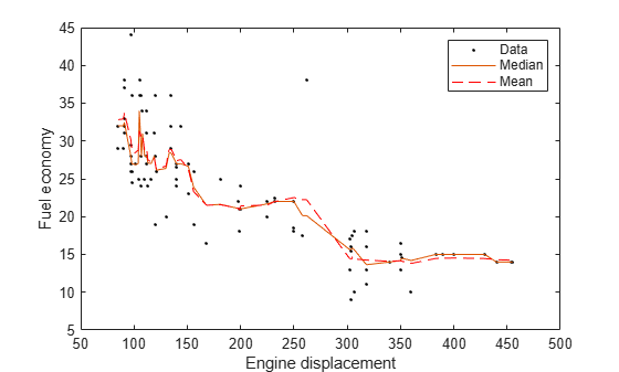
Perform quantile regression to predict the median MPG for all sorted training observations.

medianMPG = quantilePredict(Mdl,sort(Displacement));

medianMPG is an n-by-1 numeric vector of medians corresponding to the conditional distribution of the response given the sorted observations in Displacement. n is the number of observations in Displacement.

Plot the observations and the estimated medians on the same figure. Compare the median and mean responses.

meanMPG = predict(Mdl,sort(Displacement));

figure;
plot(Displacement,MPG,'k.');
hold on
plot(sort(Displacement),medianMPG);
plot(sort(Displacement),meanMPG,'r--');
ylabel('Fuel economy');
xlabel('Engine displacement');
legend('Data','Median','Mean');
hold off;

Estimate Prediction Intervals Using Percentiles

Load the carsmall data set. Consider a model that predicts the fuel economy of a car given its engine displacement.

load carsmall

Train an ensemble of bagged regression trees using the entire data set. Specify 100 weak learners.

rng(1); % For reproducibility
Mdl = TreeBagger(100,Displacement,MPG,'Method','regression');

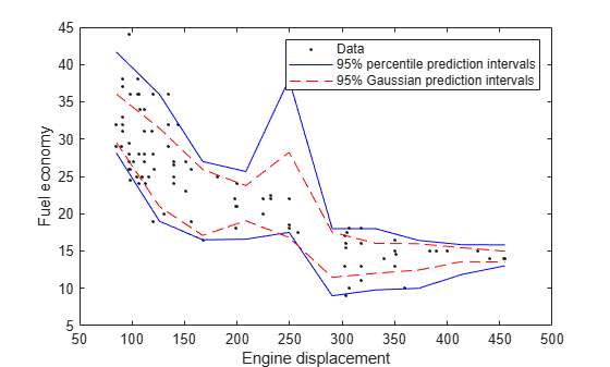
Perform quantile regression to predict the 2.5% and 97.5% percentiles for ten equally-spaced engine displacements between the minimum and maximum in-sample displacement.

predX = linspace(min(Displacement),max(Displacement),10)';
quantPredInts = quantilePredict(Mdl,predX,'Quantile',[0.025,0.975]);

quantPredInts is a 10-by-2 numeric matrix of prediction intervals corresponding to the observations in predX. The first column contains the 2.5% percentiles and the second column contains the 97.5% percentiles.

Plot the observations and the estimated medians on the same figure. Compare the percentile prediction intervals and the 95% prediction intervals assuming the conditional distribution of MPG is Gaussian.

[meanMPG,steMeanMPG] = predict(Mdl,predX);
stndPredInts = meanMPG + [-1 1]*norminv(0.975).*steMeanMPG;

figure;
h1 = plot(Displacement,MPG,'k.');
hold on
h2 = plot(predX,quantPredInts,'b');
h3 = plot(predX,stndPredInts,'r--');
ylabel('Fuel economy');
xlabel('Engine displacement');
legend([h1,h2(1),h3(1)],{'Data','95% percentile prediction intervals',...
    '95% Gaussian prediction intervals'});
hold off;

Estimate Conditional Cumulative Distribution Using Quantile Regression

Load the carsmall data set. Consider a model that predicts the fuel economy of a car given its engine displacement.

load carsmall

Train an ensemble of bagged regression trees using the entire data set. Specify 100 weak learners.

rng(1); % For reproducibility
Mdl = TreeBagger(100,Displacement,MPG,'Method','regression');

Estimate the response weights for a random sample of four training observations. Plot the training sample and identify the chosen observations.

[predX,idx] = datasample(Mdl.X,4);
[~,YW] = quantilePredict(Mdl,predX);
n = numel(Mdl.Y);

figure;
plot(Mdl.X,Mdl.Y,'o');
hold on
plot(predX,Mdl.Y(idx),'*','MarkerSize',10);
text(predX-10,Mdl.Y(idx)+1.5,{'obs. 1' 'obs. 2' 'obs. 3' 'obs. 4'});
legend('Training Data','Chosen Observations');
xlabel('Engine displacement')
ylabel('Fuel economy')
hold off

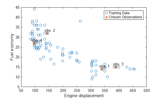
YW is an n-by-4 sparse matrix containing the response weights. Columns correspond to test observations and rows correspond to responses in the training sample. Response weights are independent of the specified quantile probability.

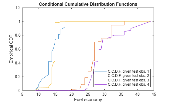
Estimate the conditional cumulative distribution function (C.C.D.F.) of the responses by:

1. Sorting the responses is ascending order, and then sorting the response weights using the indices induced by sorting the responses.

2. Computing the cumulative sums over each column of the sorted response weights.

[sortY,sortIdx] = sort(Mdl.Y);
cpdf = full(YW(sortIdx,:));
ccdf = cumsum(cpdf);

ccdf(:,j) is the empirical C.C.D.F. of the response given test observation j.

Plot the four empirical C.C.D.F. in the same figure.

figure;
plot(sortY,ccdf);
legend('C.C.D.F. given test obs. 1','C.C.D.F. given test obs. 2',...
    'C.C.D.F. given test obs. 3','C.C.D.F. given test obs. 4',...
    'Location','SouthEast')
title('Conditional Cumulative Distribution Functions')
xlabel('Fuel economy')
ylabel('Empirical CDF')

More About

Response Weights

Response weights are scalars that represent the conditional distribution of the response given a value in the predictor space. The observations in the bootstrap samples and the leaves that the training and test observations share induce response weights.

Given the observation x, the response weight for observation j in the training sample using tree t in the ensemble is

$$w_{tj}(x)=\frac{I\{X_j\in S_t(x)\}}{{\displaystyle \sum _{k=1}^{n_{\text{train}}}I\{X_k\in S_t(x)\}}},$$

where:

• I{h} is the indicator function.

• S_t(x) is the leaf of tree t containing x.

• n_train is the number of training observations.

In other words, the response weights of a particular tree form the conditional relative frequency distribution of the response.

The response weights for the entire ensemble are averaged over the trees:

$$w_j^{\ast }(x)=\frac{1}{T}{\displaystyle \sum _{t=1}^T{w}_{tj}(x)}.$$

Quantile Random Forest

Quantile random forest [2] is a quantile-regression method that uses a random forest [1] of regression trees to model the conditional distribution of a response variable, given the value of predictor variables. You can use a fitted model to estimate quantiles in the conditional distribution of the response.

Besides quantile estimation, you can use quantile regression to estimate prediction intervals or detect outliers. For example:

• To estimate 95% quantile prediction intervals, estimate the 0.025 and 0.975 quantiles.

• To detect outliers, estimate the 0.01 and 0.99 quantiles. All observations smaller than the 0.01 quantile and larger than the 0.99 quantile are outliers. All observations that are outside the interval [L,U] can be considered outliers:

  $$L=Q_1-1.5*IQR$$

  and

  $$U=Q_3+1.5*IQR,$$

  where:

  • Q₁ is the 0.25 quantile.

  • Q₃ is the 0.75 quantile.

  • IQR = Q₃ – Q₁ (the interquartile range).

Tips

quantilePredict estimates the conditional distribution of the response using the training data every time you call it. To predict many quantiles efficiently, or quantiles for many observations efficiently, you should pass X as a matrix or table of observations and specify all quantiles in a vector using the Quantile name-value pair argument. That is, avoid calling quantilePredict within a loop.

Algorithms

• The TreeBagger grows a random forest of regression trees using the training data. Then, to implement quantile random forest, quantilePredict predicts quantiles using the empirical conditional distribution of the response given an observation from the predictor variables. To obtain the empirical conditional distribution of the response:

  1. quantilePredict passes all the training observations in Mdl.X through all the trees in the ensemble, and stores the leaf nodes of which the training observations are members.

  2. quantilePredict similarly passes each observation in X through all the trees in the ensemble.

  3. For each observation in X, quantilePredict:

     1. Estimates the conditional distribution of the response by computing response weights for each tree.

     2. For observation k in X, aggregates the conditional distributions for the entire ensemble:

        $$\widehat{F}\left(y|X=x_k\right)={\displaystyle \sum _{j=1}^n{\displaystyle \sum _{t=1}^T\frac{1}{T}{w}_{tj}\left(x_k\right)}I\left\{Y_j\le y\right\}}.$$

        n is the number of training observations (size(Y,1)) and T is the number of trees in the ensemble (Mdl.NumTrees).

  4. For observation k in X, the τ quantile or, equivalently, the 100τ% percentile, is $$Q_{\tau }(x_k)=\inf \left\{y:\widehat{F}\left(y|X=x_k\right)\ge \tau \right\}.$$

• This process describes how quantilePredict uses all specified weights.

  1. For all training observations j = 1,...,n and all chosen trees t = 1,...,T,

     quantilePredict attributes the product v_tj = b_tjw_j,obs to training observation j (stored in Mdl.X(j,:) and Mdl.Y(j)). b_tj is the number of times observation j is in the bootstrap sample for tree t. w_j,obs is the observation weight in Mdl.W(j).

  2. For each chosen tree, quantilePredict identifies the leaves in which each training observation falls. Let S_t(x_j) be the set of all observations contained in the leaf of tree t of which observation j is a member.

  3. For each chosen tree, quantilePredict normalizes all weights within a particular leaf to sum to 1, that is,

     $$v_{tj}^{\ast }=\frac{v_{tj}}{{\displaystyle \sum _{i\in S_t(x_j)}{v}_{ti}}}.$$

  4. For each training observation and tree, quantilePredict incorporates tree weights (w_t,tree) specified by TreeWeights, that is, w^*_tj,tree = w_t,treev_tj^*Trees not chosen for prediction have 0 weight.

  5. For all test observations k = 1,...,K in X and all chosen trees t = 1,...,TquantilePredict predicts the unique leaves in which the observations fall, and then identifies all training observations within the predicted leaves. quantilePredict attributes the weight u_tj such that

     $$u_{tj}=\{\begin{array}{l}{w}_{tj,\text{tree}}^{\ast };\text{if }{x}_k\in S_t(x_j)\hfill \\ 0;\text{otherwise}\hfill \end{array}.$$

  6. quantilePredict sums the weights over all chosen trees, that is,

     $$u_j={\displaystyle \sum _{t=1}^T{u}_{tj}}.$$

  7. quantilePredict creates response weights by normalizing the weights so that they sum to 1, that is,

     $$w_j^{\ast }=\frac{u_j}{{\displaystyle {\sum }_{j=1}^n{u}_j}}.$$

References

[1] Breiman, L. "Random Forests." Machine Learning 45, pp. 5–32, 2001.

[2] Meinshausen, N. “Quantile Regression Forests.” Journal of Machine Learning Research, Vol. 7, 2006, pp. 983–999.

Version History

Introduced in R2016b