Set Up Multivariate Regression Problems
Response Matrix
To fit a multivariate linear regression model using mvregress,
you must set up your response matrix and design matrices in a particular way. Given
properly formatted inputs, mvregress can handle a variety of
multivariate regression problems.
mvregress expects the n observations of
potentially correlated d-dimensional responses to be in an
n-by-d matrix, named Y,
for example. That is, set up your responses so that the dependency structure is
between observations in the same row. If you specify
Y as a vector of length n (either a row or
column vector), then mvregress assumes that d
= 1, and treats the elements as n independent observations. It
does not model the vector as one realization of a correlated
series (such as a time series).
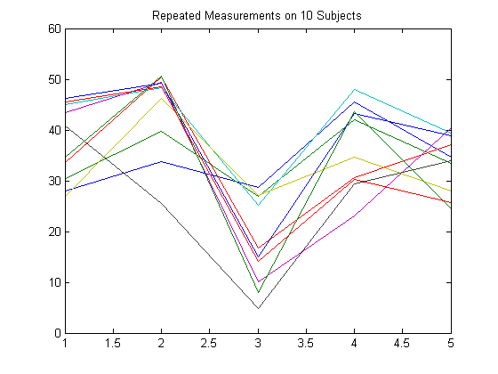
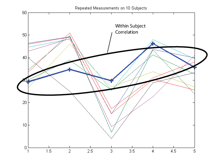
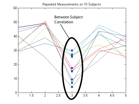
To illustrate how to set up a response matrix, suppose that your multivariate responses are repeated measurements made on subjects at multiple time points, as in the following figure.

Suppose that observations within a subject are correlated.

In this case, set up the response matrix Y such
that each row corresponds to a subject, and each column corresponds to a time point.

Then again, suppose that observations made on subjects at the same time are correlated (concurrent correlation).

In this case, set up the response matrix Y such
that each row corresponds to a time point, and each column corresponds to a subject.

Design Matrices
In the multivariate linear regression model, each d-dimensional response has a corresponding design matrix. Depending on the model, the design matrix might be comprised of exogenous predictor variables, dummy variables, lagged responses, or a combination of these and other covariate terms.
If d > 1 and all d dimensions have the same design matrix, then specify one n-by-p design matrix, where p is the number of predictor variables. To determine an intercept for each dimension, add a column of ones to the design matrix. In this case,
mvregressapplies the design matrix to all d dimensions.If d > 1 and all d dimensions do not have the same design matrix, then specify the design matrices using a length-n cell array of d-by-K arrays, named
X, for example. K is the total number of regression coefficients in the model. Note that the rows of the arrays inXcorrespond to the columns of the response matrix,Y.
If all n observations have the same design matrix, you can specify a cell array containing one d-by-K design matrix. In this case,
mvregressapplies the design matrix to all n observations. For example, this situation might arise if the predictors are functions of time, and all observations were measured at the same time points.In the special case that d = 1, you can specify one n-by-K design matrix (not in a cell array). However, you should consider using
fitlmto fit regression models to univariate, continuous responses.
The following sections illustrate how to set up the some common multivariate
regression problems for estimation using mvregress.
Common Multivariate Regression Problems
Multivariate General Linear Model
The multivariate general linear model is of the form
In expanded form,
That is, each d-dimensional response has
an intercept and p predictor variables, and each dimension
has its own set of regression coefficients. In this form, the least squares
solution is B = X\Y. To estimate this model using
mvregress, use the
n-by-d matrix of responses, as
above.
If all d dimensions have the same design matrix, use the n-by-(p+1) design matrix, as above. Adding a column of ones to the p predictor variables computes the intercept for each dimension.
If all d dimensions do not have the same design matrix, reformat the n-by-(p + 1) design matrix into a length-n cell array of d-by-K matrices. Here, K = (p + 1)d for an intercept and slopes for each dimension.
For example, suppose n = 4, d = 3, and p = 2 (two predictor terms in addition to an intercept). This figure shows how to format the ith element in the cell array.
If you prefer, you can reshape the K-by-1 vector of coefficients back into a (p + 1)-by-d matrix after estimation.
To put constraints on the model parameters, adjust the design matrix accordingly. For example, suppose that the three dimensions in the previous example have a common slope. That is, and In this case, each design matrix is 3-by-5, as shown in the following figure.
Longitudinal Analysis
In a longitudinal analysis, you might measure responses on n subjects at d time points, with correlation between observations made on the same subject. For example, suppose that you measure responses yij at times tij, i = 1,...,n and j = 1,...,d. In addition, suppose that each subject is in one of two groups (such as male or female), specified by the indicator variable Gi. You could model yij as a function of Gi and tij, with group-specific intercepts and slopes, as follows:
where
Most longitudinal models include time as an explicit predictor.
To fit this model using mvregress, arrange the responses in
an n-by-d matrix, where
n is the number of subjects and d is
the number of time points. Specify the design matrices in an
n-length cell array of
d-by-K matrices, where here
K = 4 for the four regression coefficients.
For example, suppose d = 5 (five observations per subject). The ith design matrix and corresponding parameter vector for the specified model are shown in the following figure.
Panel Analysis
In a panel analysis, you might measure responses and covariates on d subjects (such as individuals or countries) at n time points. For example, suppose you measure responses ytj and covariates xtj on subjects j = 1,...,d at times t = 1,...,n. A fixed effects panel model, with subject-specific fixed effects, and concurrent correlation might look like:
where
In contrast to longitudinal models, the panel analysis model typically includes covariates measured at each time point, instead of using time as an explicit predictor.
To fit this model using mvregress, arrange the responses in
an n-by-d matrix, such that each column
corresponds to a subject. Specify the design matrices in an
n-length cell array of
d-by-K matrices, where here
K = d + 1 for the d
intercepts and a slope term.
For example, suppose d = 4 (four subjects). The tth design matrix and corresponding parameter vector are shown in the following figure.
Seemingly Unrelated Regression
In a seemingly unrelated regression (SUR), you model d separate regressions, each with its own intercept and slope, but a common error variance-covariance matrix. For example, suppose you measure responses yij and covariates xij for regression models j = 1,...,d, with i = 1,...,n observations to fit each regression. The SUR model might look like:
where
This model is very similar to the multivariate general linear model, except that it has different covariates for each dimension.
To fit this model using mvregress, arrange the responses in
an n-by-d matrix, such that each column
has the data for the jth regression model. Specify the design
matrices in an n-length cell array of
d-by-K matrices, where here
K = 2d for d
intercepts and d slopes.
For example, suppose d = 3 (three regressions). The ith design matrix and corresponding parameter vector are shown in the following figure.
Vector Autoregressive Model
The VAR(p) vector autoregressive model expresses d-dimensional time series responses as a linear function of p lagged d-dimensional responses from previous times. For example, suppose you measure responses ytj for time series j = 1,...,d at times t = 1,...,n. The VAR(p) model might look like:
where
When estimating vector autoregressive models, you typically need to use the first p observations to initiate the model, or provide some other presample response values.
To fit this model using mvregress, arrange the responses in
an n-by-d matrix, such that each column
corresponds to a time series. Specify the design matrices in an
n-length cell array of
d-by-K matrices, where here
K = d +
pd2.
For example, suppose d = 2 (two time series) and p = 1 (one lag). The tth design matrix and corresponding parameter vector are shown in the following figure.
Alternatively, Econometrics Toolbox™ has functions for fitting and forecasting VAR(p) models, including the option to specify exogenous predictor variables.