Partial Least Squares
Introduction to Partial Least Squares
Partial least-squares (PLS) regression is a technique used with data that contain correlated predictor variables. This technique constructs new predictor variables, known as components, as linear combinations of the original predictor variables. PLS constructs these components while considering the observed response values, leading to a parsimonious model with reliable predictive power.
The technique is something of a cross between multiple linear regression and principal component analysis:
Multiple linear regression finds a combination of the predictors that best fit a response.
Principal component analysis finds combinations of the predictors with large variance, reducing correlations. The technique makes no use of response values.
PLS finds combinations of the predictors that have a large covariance with the response values.
PLS therefore combines information about the variances of both the predictors and the responses, while also considering the correlations among them.
PLS shares characteristics with other regression and feature transformation techniques. It is similar to ridge regression in that it is used in situations with correlated predictors. It is similar to stepwise regression (or more general feature selection techniques) in that it can be used to select a smaller set of model terms. PLS differs from these methods, however, by transforming the original predictor space into the new component space.
The function plsregress carries out PLS regression.
Perform Partial Least-Squares Regression
This example demonstrates how to perform PLS regression and how to choose the number of components in a PLS model.
Consider the data on biochemical oxygen demand in moore.mat, padded with noisy versions of the predictors to introduce correlations.
load moore
y = moore(:,6);              % Response
X0 = moore(:,1:5);           % Original predictors
X1 = X0+10*randn(size(X0));  % Correlated predictors
X = [X0,X1];
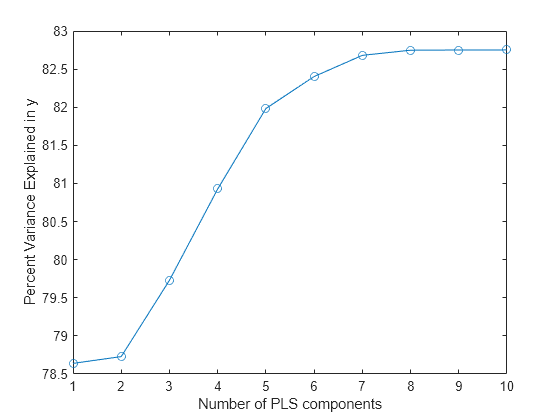
Use plsregress to perform PLS regression with the same number of components as predictors, then plot the percentage variance explained in the response as a function of the number of components.
[XL,yl,XS,YS,beta,PCTVAR] = plsregress(X,y,10);
plot(1:10,cumsum(100*PCTVAR(2,:)),'-o')
xlabel('Number of PLS components')
ylabel('Percent Variance Explained in y')

Choosing the number of components in a PLS model is a critical step. The plot gives a rough indication, showing nearly 80% of the variance in y explained by the first component, with as many as five additional components making significant contributions.
The following computes the six-component model.
[XL,yl,XS,YS,beta,PCTVAR,MSE,stats] = plsregress(X,y,6);
yfit = [ones(size(X,1),1) X]*beta;
plot(y,yfit,'o')
The scatter shows a reasonable correlation between fitted and observed responses, and this is confirmed by the statistic.
TSS = sum((y-mean(y)).^2);
RSS = sum((y-yfit).^2);
Rsquared = 1 - RSS/TSS
Rsquared =
0.8240
A plot of the weights of the ten predictors in each of the six components shows that two of the components (the last two computed) explain the majority of the variance in X.
figure
plot(1:10,stats.W,'o-')
legend({'c1','c2','c3','c4','c5','c6'},'Location','best')
xlabel('Predictor')
ylabel('Weight')

A plot of the mean-squared errors suggests that as few as two components may provide an adequate model.
figure
yyaxis left
plot(0:6,MSE(1,:),'-o')
yyaxis right
plot(0:6,MSE(2,:),'-o')
legend('MSE Predictors','MSE Response')
xlabel('Number of Components')

The calculation of mean-squared errors by plsregress is controlled by optional name-value arguments specifying cross-validation type and the number of Monte Carlo repetitions.