Mixed-Effects Models Using nlmefit and nlmefitsa
This example fits mixed-effects models, plots predictions and residuals, and interprets the results.
Load the sample data.
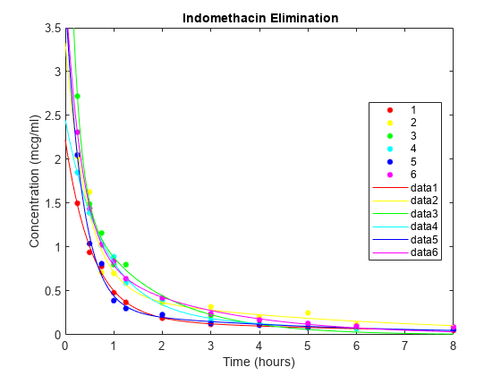
load indomethacinThe data in indomethacin.mat records concentrations of the drug indomethacin in the bloodstream of six subjects over eight hours.
Plot the scatter plot of indomethacin in the bloodstream grouped by subject.
colors = 'rygcbm';
gscatter(time,concentration,subject,colors)
xlabel('Time (hours)')
ylabel('Concentration (mcg/ml)')
title('{\bf Indomethacin Elimination}')
hold on
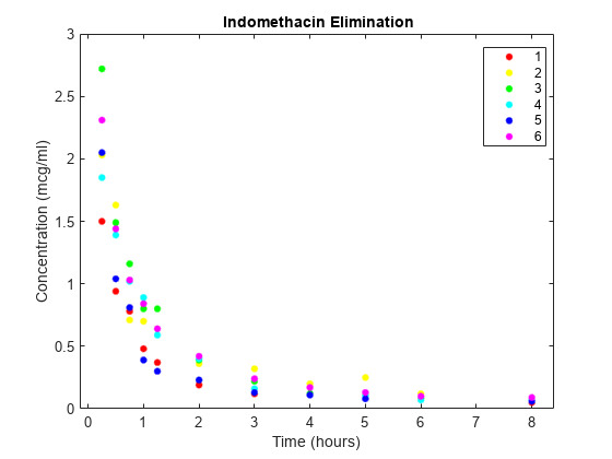
Including random effects in a model is effective when data falls into natural groups. In this data, the groups are simply the individuals under study. For details on mixed-effects models, which account for fixed effects and random effects, see Mixed-Effects Models.
Construct the model via an anonymous function.
model = @(phi,t)(phi(1)*exp(-exp(phi(2))*t) + ...
                 phi(3)*exp(-exp(phi(4))*t));
Use the nlinfit function to fit the model to all of the data, ignoring subject-specific effects.
phi0 = [1 2 1 1];
[phi,res] = nlinfit(time,concentration,model,phi0);
Compute the mean squared error.
numObs = length(time);
numParams = 4;
df = numObs-numParams;
mse = (res'*res)/df
mse =
0.0304
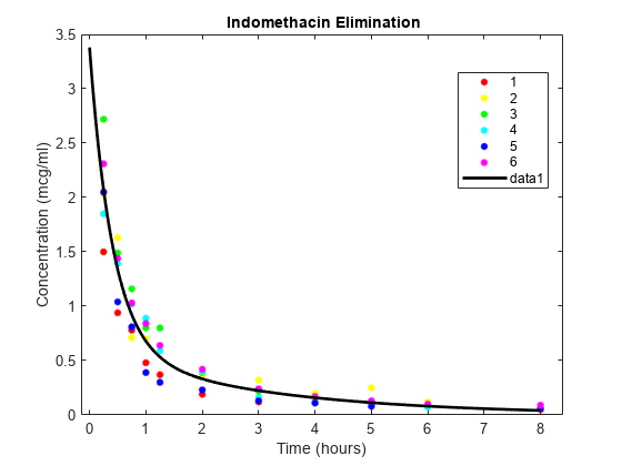
Superimpose the model on the scatter plot of data.
tplot = 0:0.01:8;
plot(tplot,model(phi,tplot),'k','LineWidth',2)
hold off
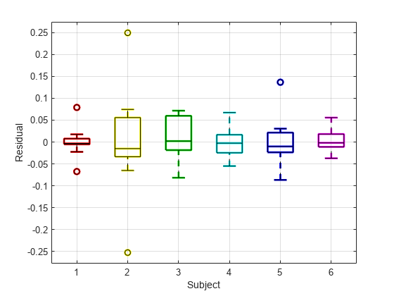
Draw the box plot of residuals by subject.
h = boxplot(res,subject,'colors',colors,'symbol','o');
set(h(~isnan(h)),'LineWidth',2)
hold on
boxplot(res,subject,'colors','k','symbol','ko')
grid on
xlabel('Subject')
ylabel('Residual')
hold off
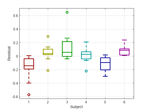
The box plot of residuals by subject shows that the boxes are mostly above or below zero, indicating that the model has failed to account for subject-specific effects.
To account for subject-specific effects, fit the model separately to the data for each subject.
phi0 = [1 2 1 1];
PHI = zeros(4,6);
RES = zeros(11,6);
for I = 1:6
    tI = time(subject == I);
    cI = concentration(subject == I);
    [PHI(:,I),RES(:,I)] = nlinfit(tI,cI,model,phi0);
end
PHI
PHI = 4×6

    2.0293    2.8277    5.4683    2.1981    3.5661    3.0023
    0.5794    0.8013    1.7498    0.2423    1.0408    1.0882
    0.1915    0.4989    1.6757    0.2545    0.2915    0.9685
   -1.7878   -1.6354   -0.4122   -1.6026   -1.5069   -0.8731
Compute the mean squared error.
numParams = 24;
df = numObs-numParams;
mse = (RES(:)'*RES(:))/df
mse =
0.0057
Plot the scatter plot of the data and superimpose the model for each subject.
gscatter(time,concentration,subject,colors)
xlabel('Time (hours)')
ylabel('Concentration (mcg/ml)')
title('{\bf Indomethacin Elimination}')
hold on
for I = 1:6
    plot(tplot,model(PHI(:,I),tplot),'Color',colors(I))
end
axis([0 8 0 3.5])
hold off
PHI gives estimates of the four model parameters for each of the six subjects. The estimates vary considerably, but taken as a 24-parameter model of the data, the mean-squared error of 0.0057 is a significant reduction from 0.0304 in the original four-parameter model.
Draw the box plot of residuals by subject.
h = boxplot(RES,'colors',colors,'symbol','o');
set(h(~isnan(h)),'LineWidth',2)
hold on
boxplot(RES,'colors','k','symbol','ko')
grid on
xlabel('Subject')
ylabel('Residual')
hold off
Now the box plot shows that the larger model accounts for most of the subject-specific effects. The spread of the residuals (the vertical scale of the box plot) is much smaller than in the previous box plot, and the boxes are now mostly centered on zero.
While the 24-parameter model successfully accounts for variations due to the specific subjects in the study, it does not consider the subjects as representatives of a larger population. The sampling distribution from which the subjects are drawn is likely more interesting than the sample itself. The purpose of mixed-effects models is to account for subject-specific variations more broadly, as random effects varying around population means.
Use the nlmefit function to fit a mixed-effects model to the data. You can also use nlmefitsa in place of nlmefit.
The following anonymous function, nlme_model , adapts the four-parameter model used by nlinfit to the calling syntax of nlmefit by allowing separate parameters for each individual. By default, nlmefit assigns random effects to all the model parameters. Also by default, nlmefit assumes a diagonal covariance matrix (no covariance among the random effects) to avoid overparameterization and related convergence issues.
nlme_model = @(PHI,t)(PHI(:,1).*exp(-exp(PHI(:,2)).*t) + ...
                      PHI(:,3).*exp(-exp(PHI(:,4)).*t));
phi0 = [1 2 1 1];
[phi,PSI,stats] = nlmefit(time,concentration,subject, ...
                          [],nlme_model,phi0)
phi = 4×1

    2.8277
    0.7729
    0.4606
   -1.3459
PSI = 4×4

    0.3264         0         0         0
         0    0.0250         0         0
         0         0    0.0124         0
         0         0         0    0.0000
stats = struct with fields:
           dfe: 57
          logl: 54.5882
           mse: 0.0066
          rmse: 0.0787
    errorparam: 0.0815
           aic: -91.1765
           bic: -93.0506
          covb: [4×4 double]
        sebeta: [0.2558 0.1066 0.1092 0.2244]
          ires: [66×1 double]
          pres: [66×1 double]
         iwres: [66×1 double]
         pwres: [66×1 double]
         cwres: [66×1 double]
The mean-squared error of 0.0066 is comparable to the 0.0057 of the 24-parameter model without random effects, and significantly better than the 0.0304 of the four-parameter model without random effects.
The estimated covariance matrix PSI shows that the variance of the fourth random effect is essentially zero, suggesting that you can remove it to simplify the model. To do this, use the 'REParamsSelect' name-value pair to specify the indices of the parameters to be modeled with random effects in nlmefit.
[phi,PSI,stats] = nlmefit(time,concentration,subject, ...
                          [],nlme_model,phi0, ...
                          'REParamsSelect',[1 2 3])
phi = 4×1

    2.8277
    0.7728
    0.4605
   -1.3460
PSI = 3×3

    0.3270         0         0
         0    0.0250         0
         0         0    0.0124
stats = struct with fields:
           dfe: 58
          logl: 54.5875
           mse: 0.0066
          rmse: 0.0780
    errorparam: 0.0815
           aic: -93.1750
           bic: -94.8410
          covb: [4×4 double]
        sebeta: [0.2560 0.1066 0.1092 0.2244]
          ires: [66×1 double]
          pres: [66×1 double]
         iwres: [66×1 double]
         pwres: [66×1 double]
         cwres: [66×1 double]
The log-likelihood logl is almost identical to what it was with random effects for all of the parameters, the Akaike information criterion aic is reduced from -91.1765 to -93.1750, and the Bayesian information criterion bic is reduced from -93.0506 to -94.8410. These measures support the decision to drop the fourth random effect.
Refitting the simplified model with a full covariance matrix allows for identification of correlations among the random effects. To do this, use the CovPattern parameter to specify the pattern of nonzero elements in the covariance matrix.
[phi,PSI,stats] = nlmefit(time,concentration,subject, ...
                          [],nlme_model,phi0, ...
                          'REParamsSelect',[1 2 3], ...
                          'CovPattern',ones(3))
phi = 4×1

    2.8149
    0.8292
    0.5612
   -1.1410
PSI = 3×3

    0.4768    0.1152    0.0500
    0.1152    0.0321    0.0032
    0.0500    0.0032    0.0236
stats = struct with fields:
           dfe: 55
          logl: 58.4721
           mse: 0.0061
          rmse: 0.0782
    errorparam: 0.0781
           aic: -94.9442
           bic: -97.2348
          covb: [4×4 double]
        sebeta: [0.3028 0.1104 0.1179 0.1662]
          ires: [66×1 double]
          pres: [66×1 double]
         iwres: [66×1 double]
         pwres: [66×1 double]
         cwres: [66×1 double]
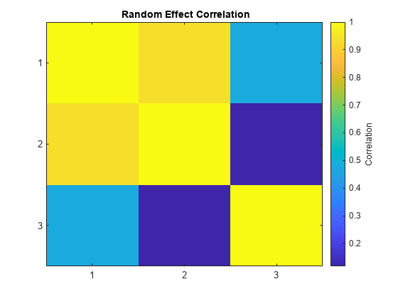
The estimated covariance matrix PSI shows that the random effects on the first two parameters have a relatively strong correlation, and both have a relatively weak correlation with the last random effect. This structure in the covariance matrix is more apparent if you convert PSI to a correlation matrix using corrcov.
RHO = corrcov(PSI)
RHO = 3×3

    1.0000    0.9315    0.4711
    0.9315    1.0000    0.1179
    0.4711    0.1179    1.0000
clf;
imagesc(RHO)
set(gca,'XTick',[1 2 3],'YTick',[1 2 3])
title('{\bf Random Effect Correlation}')
h = colorbar;
set(get(h,'YLabel'),'String','Correlation');
Incorporate this structure into the model by changing the specification of the covariance pattern to block-diagonal.
P = [1 1 0;1 1 0;0 0 1] % Covariance patternP = 3×3
1 1 0
1 1 0
0 0 1
[phi,PSI,stats,b] = nlmefit(time,concentration,subject, ...
                            [],nlme_model,phi0, ...
                            'REParamsSelect',[1 2 3], ...
                            'CovPattern',P)
phi = 4×1

    2.7830
    0.8981
    0.6581
   -1.0000
PSI = 3×3

    0.5180    0.1069         0
    0.1069    0.0221         0
         0         0    0.0454
stats = struct with fields:
           dfe: 57
          logl: 58.0804
           mse: 0.0061
          rmse: 0.0768
    errorparam: 0.0782
           aic: -98.1608
           bic: -100.0350
          covb: [4×4 double]
        sebeta: [0.3171 0.1073 0.1384 0.1453]
          ires: [66×1 double]
          pres: [66×1 double]
         iwres: [66×1 double]
         pwres: [66×1 double]
         cwres: [66×1 double]
b = 3×6

   -0.8507   -0.1563    1.0427   -0.7559    0.5652    0.1550
   -0.1756   -0.0323    0.2152   -0.1560    0.1167    0.0320
   -0.2756    0.0519    0.2620    0.1064   -0.2835    0.1389
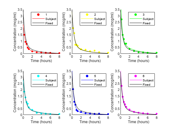
The block-diagonal covariance structure reduces aic from -94.9462 to -98.1608 and bic from -97.2368 to -100.0350 without significantly affecting the log-likelihood. These measures support the covariance structure used in the final model. The output b gives predictions of the three random effects for each of the six subjects. These are combined with the estimates of the fixed effects in phi to produce the mixed-effects model.
Plot the mixed-effects model for each of the six subjects. For comparison, the model without random effects is also shown.
PHI = repmat(phi,1,6) + ...                 % Fixed effects
      [b(1,:);b(2,:);b(3,:);zeros(1,6)];    % Random effects
RES = zeros(11,6); % Residuals
colors = 'rygcbm';
for I = 1:6
    fitted_model = @(t)(PHI(1,I)*exp(-exp(PHI(2,I))*t) + ...
                        PHI(3,I)*exp(-exp(PHI(4,I))*t));
    tI = time(subject == I);
    cI = concentration(subject == I);
    RES(:,I) = cI - fitted_model(tI);

    subplot(2,3,I)
    scatter(tI,cI,20,colors(I),'filled')
    hold on
    plot(tplot,fitted_model(tplot),'Color',colors(I))
    plot(tplot,model(phi,tplot),'k')
    axis([0 8 0 3.5])
    xlabel('Time (hours)')
    ylabel('Concentration (mcg/ml)')
    legend(num2str(I),'Subject','Fixed')
end
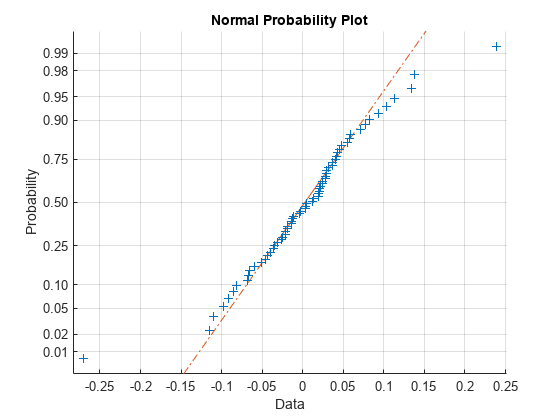
If obvious outliers in the data (visible in previous box plots) are ignored, a normal probability plot of the residuals shows reasonable agreement with model assumptions on the errors.
figure
normplot(RES(:))