incrementalRegressionKernel
Description
The incrementalRegressionKernel function creates an
incrementalRegressionKernel model object, which represents a binary Gaussian kernel
regression model for incremental learning. The kernel model maps data in a low-dimensional
space into a high-dimensional space, then fits a linear model in the high-dimensional space.
Supported linear models include support vector machine (SVM) and least-squares
regression.
Unlike other Statistics and Machine Learning Toolbox™ model objects, incrementalRegressionKernel can be called directly. Also,
you can specify learning options, such as performance metrics configurations and the objective
solver, before fitting the model to data. After you create an incrementalRegressionKernel
object, it is prepared for incremental learning.
incrementalRegressionKernel is best suited for incremental learning. For a traditional
approach to training a kernel regression model (such as creating a model by fitting it to
data, performing cross-validation, tuning hyperparameters, and so on), see fitrkernel.
Creation
You can create an incrementalRegressionKernel model object in several ways:
Call the function directly — Configure incremental learning options, or specify learner-specific options, by calling
incrementalRegressionKerneldirectly. This approach is best when you do not have data yet or you want to start incremental learning immediately.Convert a traditionally trained model — To initialize a model for incremental learning using the model parameters and hyperparameters of a trained model object (
RegressionKernel), you can convert the traditionally trained model to anincrementalRegressionKernelmodel object by passing it to theincrementalLearnerfunction.Call an incremental learning function —
fit,updateMetrics, andupdateMetricsAndFitaccept a configuredincrementalRegressionKernelmodel object and data as input, and return anincrementalRegressionKernelmodel object updated with information learned from the input model and data.
Description
Mdl = incrementalRegressionKernel()Mdl. Properties of a default model contain placeholders for unknown
model parameters. You must train a default model before you can track its performance or
generate predictions from it.
Mdl = incrementalRegressionKernel(Name=Value)incrementalRegressionKernel(Solver="sgd",LearnRateSchedule="constant")
specifies to use the stochastic gradient descent (SGD) solver with a constant learning
rate.
Name-Value Arguments
Properties
Object Functions
fit | Train kernel model for incremental learning |
updateMetrics | Update performance metrics in kernel incremental learning model given new data |
updateMetricsAndFit | Update performance metrics in kernel incremental learning model given new data and train model |
loss | Loss of kernel incremental learning model on batch of data |
predict | Predict responses for new observations from kernel incremental learning model |
perObservationLoss | Per observation regression error of model for incremental learning |
reset | Reset incremental regression model |
Examples
Create an incremental kernel model without any prior information. Track the model performance on streaming data, and fit the model to the data.
Create a default incremental kernel SVM model for regression.
Mdl = incrementalRegressionKernel()
Mdl =
  incrementalRegressionKernel

                    IsWarm: 0
                   Metrics: [1×2 table]
         ResponseTransform: 'none'
    NumExpansionDimensions: 0
               KernelScale: 1


  Properties, Methods
Mdl.EstimationPeriod
ans =
1000
Mdl is an incrementalRegressionKernel model object. All its properties are read-only.
Mdl must be fit to data before you can use it to perform any other operations. The software sets the estimation period to 1000 because half the width of the epsilon insensitive band Epsilon is unknown. You can set Epsilon to a positive floating-point scalar by using the Epsilon name-value argument. This action results in a default estimation period of 0.
Load the robot arm data set.
load robotarmFor details on the data set, enter Description at the command line.
Fit the incremental model to the training data by using the updateMetricsAndFit function. To simulate a data stream, fit the model in chunks of 50 observations at a time. At each iteration:
Process 50 observations.
Overwrite the previous incremental model with a new one fitted to the incoming observations.
Store the cumulative metrics, window metrics, and number of training observations to see how they evolve during incremental learning.
% Preallocation
n = numel(ytrain);
numObsPerChunk = 50;
nchunk = floor(n/numObsPerChunk);
ei = array2table(zeros(nchunk,2),VariableNames=["Cumulative","Window"]);
numtrainobs = zeros(nchunk+1,1);

% Incremental fitting
for j = 1:nchunk
    ibegin = min(n,numObsPerChunk*(j-1) + 1);
    iend   = min(n,numObsPerChunk*j);
    idx = ibegin:iend;
    Mdl = updateMetricsAndFit(Mdl,Xtrain(idx,:),ytrain(idx));
    ei{j,:} = Mdl.Metrics{"EpsilonInsensitiveLoss",:};
    numtrainobs(j+1) = Mdl.NumTrainingObservations;
end
Mdl is an incrementalRegressionKernel model object trained on all the data in the stream. While updateMetricsAndFit processes the first 1000 observations, it stores the response values to estimate Epsilon; the function does not fit the model until after this estimation period. During incremental learning and after the model is warmed up, updateMetricsAndFit checks the performance of the model on the incoming observations, and then fits the model to those observations.
Plot a trace plot of the number of training observations and the performance metrics on separate tiles.
t = tiledlayout(2,1);
nexttile
plot(numtrainobs)
xlim([0 nchunk])
ylabel("Number of Training Observations")
xline(Mdl.EstimationPeriod/numObsPerChunk,"-.")
xline((Mdl.EstimationPeriod + Mdl.MetricsWarmupPeriod)/numObsPerChunk,"--")
nexttile
plot(ei.Variables)
xlim([0 nchunk])
ylabel("Epsilon Insensitive Loss")
xline(Mdl.EstimationPeriod/numObsPerChunk,"-.")
xline((Mdl.EstimationPeriod + Mdl.MetricsWarmupPeriod)/numObsPerChunk,"--")
legend(ei.Properties.VariableNames,Location="best")
xlabel(t,"Iteration")
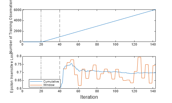
The plot suggests that updateMetricsAndFit does the following:
After the estimation period (first 20 iterations), fit the model during all incremental learning iterations.
Compute the performance metrics after the metrics warm-up period only.
Compute the cumulative metrics during each iteration.
Compute the window metrics after processing 200 observations (4 iterations).
Prepare an incremental regression learner by specifying a metrics warm-up period and a metrics window size. Train the model by using SGD, and adjust the SGD batch size, learning rate, and regularization parameter.
Load the robot arm data set.
load robotarm
n = numel(ytrain);
For details on the data set, enter Description at the command line.
Create an incremental kernel model for regression. Configure the model as follows:
Specify the SGD solver.
Assume that these settings work well for the problem: a ridge regularization parameter value of 0.001, SGD batch size of 20, learning rate of 0.002, and half the width of the epsilon insensitive band for SVM of 0.05.
Specify a metrics warm-up period of 1000 observations.
Specify a metrics window size of 500 observations.
Track the epsilon insensitive loss, MSE, and mean absolute error (MAE) to measure the performance of the model. The software supports epsilon insensitive loss and MSE. Create an anonymous function that measures the absolute error of each new observation. Create a structure array containing the name
MeanAbsoluteErrorand its corresponding function.
maefcn = @(z,zfit)abs(z - zfit);
maemetric = struct("MeanAbsoluteError",maefcn);

Mdl = incrementalRegressionKernel(Solver="sgd", ...
    Lambda=0.001,BatchSize=20,LearnRate=0.002,Epsilon=0.05, ...
    MetricsWarmupPeriod=1000,MetricsWindowSize=500, ...
    Metrics={"epsiloninsensitive","mse",maemetric})
Mdl =
  incrementalRegressionKernel

                    IsWarm: 0
                   Metrics: [3×2 table]
         ResponseTransform: 'none'
    NumExpansionDimensions: 0
               KernelScale: 1


  Properties, Methods
Mdl is an incrementalRegressionKernel model object configured for incremental learning without an estimation period.
Fit the incremental model to the data by using the updateMetricsAndFit function. At each iteration:
Simulate a data stream by processing a chunk of 50 observations. Note that the chunk size is different from the SGD batch size.
Overwrite the previous incremental model with a new one fitted to the incoming observations.
Store the cumulative metrics, window metrics, and number of training observations to see how they evolve during incremental learning.
% Preallocation
numObsPerChunk = 50;
nchunk = floor(n/numObsPerChunk);
ei = array2table(zeros(nchunk,2),VariableNames=["Cumulative","Window"]);
mse = array2table(zeros(nchunk,2),VariableNames=["Cumulative","Window"]);
mae = array2table(zeros(nchunk,2),VariableNames=["Cumulative","Window"]);
numtrainobs = zeros(nchunk,1);

% Incremental fitting
rng("default") % For reproducibility
for j = 1:nchunk
    ibegin = min(n,numObsPerChunk*(j-1) + 1);
    iend   = min(n,numObsPerChunk*j);
    idx = ibegin:iend;
    Mdl = updateMetricsAndFit(Mdl,Xtrain(idx,:),ytrain(idx));
    ei{j,:} = Mdl.Metrics{"EpsilonInsensitiveLoss",:};
    mse{j,:} = Mdl.Metrics{"MeanSquaredError",:};
    mae{j,:} = Mdl.Metrics{"MeanAbsoluteError",:};
    numtrainobs(j) = Mdl.NumTrainingObservations;
end
Mdl is an incrementalRegressionKernel model object trained on all the data in the stream. During incremental learning and after the model is warmed up, updateMetricsAndFit checks the performance of the model on the incoming observations, and then fits the model to those observations.
Plot a trace plot of the number of training observations and the performance metrics on separate tiles.
t = tiledlayout(4,1);
nexttile
plot(numtrainobs)
xlim([0 nchunk])
ylabel(["Number of","Training Observations"])
xline(Mdl.MetricsWarmupPeriod/numObsPerChunk,"--")
nexttile
plot(ei.Variables)
xlim([0 nchunk])
ylabel(["Epsilon Insensitive","Loss"])
xline(Mdl.MetricsWarmupPeriod/numObsPerChunk,"--")
legend(ei.Properties.VariableNames)
nexttile
plot(mse.Variables)
xlim([0 nchunk])
ylabel("MSE")
xline(Mdl.MetricsWarmupPeriod/numObsPerChunk,"--")
legend(mse.Properties.VariableNames)
nexttile
plot(mae.Variables)
xlim([0 nchunk])
ylabel("MAE")
xline(Mdl.MetricsWarmupPeriod/numObsPerChunk,"--")
legend(mae.Properties.VariableNames)
xlabel(t,"Iteration")
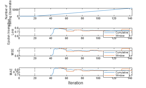
The plot suggests that updateMetricsAndFit does the following:
Fit the model during all incremental learning iterations.
Compute the performance metrics after the metrics warm-up period only.
Compute the cumulative metrics during each iteration.
Compute the window metrics after processing 500 observations (10 iterations).
Train a kernel regression model by using fitrkernel, convert it to an incremental learner, track its performance, and fit it to streaming data. Carry over training options from traditional to incremental learning.
Load and Preprocess Data
Load the 2015 NYC housing data set, and shuffle the data. For more details on the data, see NYC Open Data.
load NYCHousing2015
rng(1) % For reproducibility
n = size(NYCHousing2015,1);
idxshuff = randsample(n,n);
NYCHousing2015 = NYCHousing2015(idxshuff,:);
Suppose that the data collected from Manhattan (BOROUGH = 1) was collected using a new method that doubles its quality. Create a weight variable that attributes 2 to observations collected from Manhattan, and 1 to all other observations.
NYCHousing2015.W = ones(n,1) + (NYCHousing2015.BOROUGH == 1);
Extract the response variable SALEPRICE from the table. For numerical stability, scale SALEPRICE by 1e6.
Y = NYCHousing2015.SALEPRICE/1e6;
NYCHousing2015.SALEPRICE = [];
To reduce computational cost for this example, remove the NEIGHBORHOOD column, which contains a categorical variable with 254 categories.
NYCHousing2015.NEIGHBORHOOD = [];
Create dummy variable matrices from the other categorical predictors.
catvars = ["BOROUGH","BUILDINGCLASSCATEGORY"];
dumvarstbl = varfun(@(x)dummyvar(categorical(x)),NYCHousing2015, ...
    InputVariables=catvars);
dumvarmat = table2array(dumvarstbl);
NYCHousing2015(:,catvars) = [];
Treat all other numeric variables in the table as predictors of sales price. Concatenate the matrix of dummy variables to the rest of the predictor data.
idxnum = varfun(@isnumeric,NYCHousing2015,OutputFormat="uniform");
X = [dumvarmat NYCHousing2015{:,idxnum}];
Train Kernel Regression Model
Fit a kernel regression model to a random sample of half the data. Specify the observation weights.
idxtt = randsample([true false],n,true);
Mdl = fitrkernel(X(idxtt,:),Y(idxtt),Weights=NYCHousing2015.W(idxtt))
Mdl =
  RegressionKernel
              ResponseName: 'Y'
                   Learner: 'svm'
    NumExpansionDimensions: 2048
               KernelScale: 1
                    Lambda: 2.1977e-05
             BoxConstraint: 1
                   Epsilon: 0.0547


  Properties, Methods
Mdl is a RegressionKernel model object representing a traditionally trained kernel regression model.
Convert Trained Model
Convert the traditionally trained kernel regression model to a model for incremental learning.
IncrementalMdl = incrementalLearner(Mdl)
IncrementalMdl =
  incrementalRegressionKernel

                    IsWarm: 1
                   Metrics: [1×2 table]
         ResponseTransform: 'none'
    NumExpansionDimensions: 2048
               KernelScale: 1


  Properties, Methods
IncrementalMdl is an incrementalRegressionKernel model object configured for incremental learning.
Separately Track Performance Metrics and Fit Model
Perform incremental learning on the rest of the data by using the updateMetrics and fit functions. Simulate a data stream by processing 500 observations at a time. At each iteration:
Call
updateMetricsto update the cumulative and window epsilon insensitive loss of the model given the incoming chunk of observations. Overwrite the previous incremental model to update theMetricsproperty. Note that the function does not fit the model to the chunk of data—the chunk is "new" data for the model. Specify the observation weights.Call
fitto fit the model to the incoming chunk of observations. Overwrite the previous incremental model to update the model parameters. Specify the observation weights.Store the losses and number of training observations.
% Preallocation
idxil = ~idxtt;
nil = sum(idxil);
numObsPerChunk = 500;
nchunk = floor(nil/numObsPerChunk);
ei = array2table(zeros(nchunk,2),VariableNames=["Cumulative","Window"]);
numtrainobs = zeros(nchunk,1);
Xil = X(idxil,:);
Yil = Y(idxil);
Wil = NYCHousing2015.W(idxil);

% Incremental fitting
for j = 1:nchunk
    ibegin = min(nil,numObsPerChunk*(j-1) + 1);
    iend   = min(nil,numObsPerChunk*j);
    idx = ibegin:iend;
    IncrementalMdl = updateMetrics(IncrementalMdl,Xil(idx,:),Yil(idx), ...
        Weights=Wil(idx));
    ei{j,:} = IncrementalMdl.Metrics{"EpsilonInsensitiveLoss",:};
    IncrementalMdl = fit(IncrementalMdl,Xil(idx,:),Yil(idx), ...
        Weights=Wil(idx));
    numtrainobs(j) = IncrementalMdl.NumTrainingObservations;
end
IncrementalMdl is an incrementalRegressionKernel model object trained on all the data in the stream.
Alternatively, you can use updateMetricsAndFit to update performance metrics of the model given a new chunk of data, and then fit the model to the data.
Plot a trace plot of the number of training observations and the performance metrics on separate tiles.
t = tiledlayout(2,1);
nexttile
plot(numtrainobs)
xlim([0 nchunk])
ylabel("Number of Training Observations")
nexttile
plot(ei.Variables)
xlim([0 nchunk])
ylabel("Epsilon Insensitive Loss")
legend(ei.Properties.VariableNames)
xlabel(t,"Iteration")
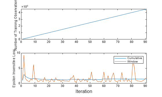
The cumulative loss gradually changes with each iteration (chunk of 500 observations), whereas the window loss jumps. Because the metrics window is 200 by default, updateMetrics measures the performance based on the latest 200 observations in each 500 observation chunk.