fitrqnet
Syntax
Description
Mdl = fitrqnet(Tbl,ResponseVarName)Mdl. The
function trains the model using the predictors in the table Tbl and the
response values in the ResponseVarName table variable.
By default, the function uses the median (0.5 quantile).
Mdl = fitrqnet(___,Name=Value)Quantiles name-value argument.
[
also returns Mdl,AggregateOptimizationResults] = fitrqnet(___)AggregateOptimizationResults, which contains
hyperparameter optimization results when you specify the
OptimizeHyperparameters and
HyperparameterOptimizationOptions name-value arguments. You must also
specify the ConstraintType and ConstraintBounds
options of HyperparameterOptimizationOptions. You can use this syntax
to optimize on the compact model size instead of the cross-validation loss, and to solve a
set of multiple optimization problems that have the same options but different constraint
bounds. (since R2025a)
Examples
Fit a quantile neural network regression model using the 0.25, 0.50, and 0.75 quantiles.
Load the carbig data set, which contains measurements of cars made in the 1970s and early 1980s. Create a matrix X containing the predictor variables Acceleration, Displacement, Horsepower, and Weight. Store the response variable MPG in the variable Y.
load carbig
X = [Acceleration,Displacement,Horsepower,Weight];
Y = MPG;
Delete rows of X and Y where either array has missing values.
R = rmmissing([X Y]);
X = R(:,1:end-1);
Y = R(:,end);
Partition the data into training data (XTrain and YTrain) and test data (XTest and YTest). Reserve approximately 20% of the observations for testing, and use the rest of the observations for training.
rng(0,"twister") % For reproducibility of the partition
c = cvpartition(length(Y),"Holdout",0.20);

trainingIdx = training(c);
XTrain = X(trainingIdx,:);
YTrain = Y(trainingIdx);

testIdx = test(c);
XTest = X(testIdx,:);
YTest = Y(testIdx);
Train a quantile neural network regression model. Specify to use the 0.25, 0.50, and 0.75 quantiles (that is, the lower quartile, median, and upper quartile). To improve the model fit, standardize the numeric predictors. Use a ridge (L2) regularization term of 0.05. Adding a regularization term can help prevent quantile crossing.
Mdl = fitrqnet(XTrain,YTrain,Quantiles=[0.25,0.50,0.75], ...
    Standardize=true,Lambda=0.05)
Mdl =
RegressionQuantileNeuralNetwork
ResponseName: 'Y'
CategoricalPredictors: []
LayerSizes: 10
Activations: 'relu'
OutputLayerActivation: 'none'
Quantiles: [0.2500 0.5000 0.7500]
Properties, Methods
Mdl is a RegressionQuantileNeuralNetwork model object. You can use dot notation to access the properties of Mdl. For example, Mdl.LayerWeights and Mdl.LayerBiases contain the weights and biases, respectively, for the fully connected layers of the trained model.
In this example, you can use the layer weights, layer biases, predictor means, and predictor standard deviations directly to predict the test set responses for each of the three quantiles in Mdl.Quantiles. In general, you can use the predict object function to make quantile predictions.
firstFCStep = (Mdl.LayerWeights{1})*((XTest-Mdl.Mu)./Mdl.Sigma)' ...
    + Mdl.LayerBiases{1};
reluStep = max(firstFCStep,0);
finalFCStep = (Mdl.LayerWeights{end})*reluStep + Mdl.LayerBiases{end};
predictedY = finalFCStep'
predictedY = 78×3
13.9602 15.1340 16.6884
11.2792 12.2332 13.4849
19.5525 21.7303 23.9473
22.6950 25.5260 28.1201
10.4533 11.3377 12.4984
17.6935 19.5194 21.5152
12.4312 13.4797 14.8614
11.7998 12.7963 14.1071
16.6860 18.3305 20.2070
24.1142 27.0301 29.7811
22.2832 25.1327 27.6841
12.8749 13.9594 15.3917
12.2328 13.2643 14.6245
24.0164 26.9150 29.6545
13.4641 14.5970 16.0957
⋮
isequal(predictedY,predict(Mdl,XTest))
ans = logical
   1
Each column of predictedY corresponds to a separate quantile (0.25, 0.5, or 0.75).
Visualize the predictions of the quantile neural network regression model. First, create a grid of predictor values.
minX = floor(min(X))
minX = 1×4

           8          68          46        1613
maxX = ceil(max(X))
maxX = 1×4

          25         455         230        5140
gridX = zeros(100,size(X,2));
for p = 1:size(X,2)
    gridp = linspace(minX(p),maxX(p))';
    gridX(:,p) = gridp;
end
Next, use the trained model Mdl to predict the response values for the grid of predictor values.
gridY = predict(Mdl,gridX)
gridY = 100×3

   31.2419   35.0661   38.6357
   30.8637   34.6317   38.1573
   30.4854   34.1972   37.6789
   30.1072   33.7627   37.2005
   29.7290   33.3283   36.7221
   29.3507   32.8938   36.2436
   28.9725   32.4593   35.7652
   28.5943   32.0249   35.2868
   28.2160   31.5904   34.8084
   27.8378   31.1560   34.3300
   27.4596   30.7215   33.8516
   27.0814   30.2870   33.3732
   26.7031   29.8526   32.8948
   26.3249   29.4181   32.4164
   25.9467   28.9837   31.9380
      ⋮
For each observation in gridX, the predict object function returns predictions for the quantiles in Mdl.Quantiles.
View the gridY predictions for the second predictor (Displacement). Compare the quantile predictions to the true test data values.
predictorIdx = 2;
plot(XTest(:,predictorIdx),YTest,".")
hold on
plot(gridX(:,predictorIdx),gridY(:,1))
plot(gridX(:,predictorIdx),gridY(:,2))
plot(gridX(:,predictorIdx),gridY(:,3))
hold off
xlabel("Predictor (Displacement)")
ylabel("Response (MPG)")
legend(["True values","0.25 predicted values", ...
    "0.50 predicted values","0.75 predicted values"])
title("Test Data")
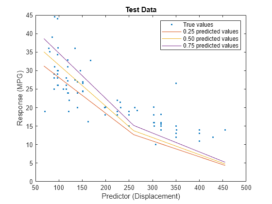
The red curve shows the predictions for the 0.25 quantile, the yellow curve shows the predictions for the 0.50 quantile, and the purple curve shows the predictions for the 0.75 quantile. The blue points indicate the true test data values.
Notice that the quantile prediction curves do not cross each other.
When training a quantile neural network regression model, you can use a ridge (L2) regularization term to prevent quantile crossing.
Load the carbig data set, which contains measurements of cars made in the 1970s and early 1980s. Create a table containing the predictor variables Acceleration, Cylinders, Displacement, and so on, as well as the response variable MPG.
load carbig
cars = table(Acceleration,Cylinders,Displacement, ...
    Horsepower,Model_Year,Origin,Weight,MPG);
Remove rows of cars where the table has missing values.
cars = rmmissing(cars);
Categorize the cars based on whether they were made in the USA.
cars.Origin = categorical(cellstr(cars.Origin));
cars.Origin = mergecats(cars.Origin,["France","Japan",...
    "Germany","Sweden","Italy","England"],"NotUSA");
Partition the data into training and test sets using cvpartition. Use approximately 80% of the observations as training data, and 20% of the observations as test data.
rng(0,"twister") % For reproducibility of the data partition
c = cvpartition(height(cars),"Holdout",0.20);

trainingIdx = training(c);
carsTrain = cars(trainingIdx,:);

testIdx = test(c);
carsTest = cars(testIdx,:);
Train a quantile neural network regression model. Use the 0.25, 0.50, and 0.75 quantiles (that is, the lower quartile, median, and upper quartile). To improve the model fit, standardize the numeric predictors before training.
Mdl = fitrqnet(carsTrain,"MPG",Quantiles=[0.25 0.5 0.75], ...
    Standardize=true);
Mdl is a RegressionNeuralNetwork model object.
Determine if the test data predictions for the quantiles in Mdl.Quantiles cross each other by using the predict object function of Mdl. The crossingIndicator output argument contains a value of 1 (true) for any observation with quantile predictions that cross.
[~,crossingIndicator] = predict(Mdl,carsTest);
sum(crossingIndicator)
ans =
2
In this example, two of the observations in carsTest have quantile predictions that cross each other.
To prevent quantile crossing, specify the Lambda name-value argument in the call to fitrqnet. Use a 0.05 ridge (L2) penalty term.
newMdl = fitrqnet(carsTrain,"MPG",Quantiles=[0.25 0.5 0.75], ...
    Standardize=true,Lambda=0.05);
[predictedY,newCrossingIndicator] = predict(newMdl,carsTest);
sum(newCrossingIndicator)
ans =
0
With regularization, the predictions for the test data set do not cross for any observations.
Visualize the predictions returned by newMdl by using a scatter plot with a reference line. Plot the predicted values along the vertical axis and the true response values along the horizontal axis. Points on the reference line indicate correct predictions.
plot(carsTest.MPG,predictedY(:,1),".")
hold on
plot(carsTest.MPG,predictedY(:,2),".")
plot(carsTest.MPG,predictedY(:,3),".")
plot(carsTest.MPG,carsTest.MPG)
hold off
xlabel("True MPG")
ylabel("Predicted MPG")
legend(["0.25 quantile values","0.50 quantile values", ...
    "0.75 quantile values","Reference line"], ...
    Location="southeast")
title("Test Data")
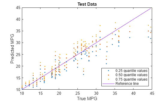
Blue points correspond to the 0.25 quantile, red points correspond to the 0.50 quantile, and yellow points correspond to the 0.75 quantile.
For a more in-depth example, see Regularize Quantile Regression Model to Prevent Quantile Crossing.
Optimize the hyperparameters of a quantile neural network regression model. Compare the test set losses of the model before and after hyperparameter optimization.
Load the carbig data set, which contains measurements of cars made in the 1970s and early 1980s. Create a table containing the predictor variables Acceleration, Cylinders, Displacement, and so on, as well as the response variable MPG. View the first eight observations.
load carbig
cars = table(Acceleration,Cylinders,Displacement, ...
    Horsepower,Model_Year,Origin,Weight,MPG);
head(cars)
    Acceleration    Cylinders    Displacement    Horsepower    Model_Year    Origin     Weight    MPG
    ____________    _________    ____________    __________    __________    _______    ______    ___

          12            8            307            130            70        USA         3504     18
        11.5            8            350            165            70        USA         3693     15
          11            8            318            150            70        USA         3436     18
          12            8            304            150            70        USA         3433     16
        10.5            8            302            140            70        USA         3449     17
          10            8            429            198            70        USA         4341     15
           9            8            454            220            70        USA         4354     14
         8.5            8            440            215            70        USA         4312     14
Remove rows of cars where the table has missing values.
cars = rmmissing(cars);
Categorize the cars based on whether they were made in the USA.
cars.Origin = categorical(cellstr(cars.Origin));
cars.Origin = mergecats(cars.Origin,["France","Japan",...
    "Germany","Sweden","Italy","England"],"NotUSA");
Partition the data into training and test sets using cvpartition. Use approximately 80% of the observations as training data, and 20% of the observations as test data.
rng(0,"twister") % For reproducibility of the data partition
c = cvpartition(height(cars),Holdout=0.20);

trainingIdx = training(c);
carsTrain = cars(trainingIdx,:);

testIdx = test(c);
carsTest = cars(testIdx,:);
Train a quantile neural network regression model using the carsTrain training data. Specify MPG as the response variable, and use the 0.05 and 0.95 quantiles. Then, compute the quantile losses using the carsTest test data.
Mdl = fitrqnet(carsTrain,"MPG",Quantiles=[0.05 0.95]);
L = loss(Mdl,carsTest)
L = 1×2
0.3445 0.4586
L(1) is the quantile loss for the 0.05 quantile, and L(2) is the quantile loss for the 0.95 quantile.
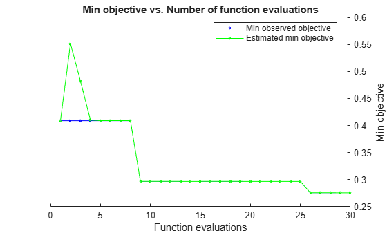
Optimize the hyperparameters of the quantile regression model using Bayesian optimization. Set OptimizeHyperparameters to "auto", which is equivalent to ["Activations","Lambda","LayerSizes","Standardize"]. By default, fitrqnet searches for the hyperparameter values that optimize the 5-fold cross-validation quantile loss, averaged across the quantiles.
optMdl = fitrqnet(carsTrain,"MPG",Quantiles=[0.05 0.95], ... OptimizeHyperparameters="auto");
|============================================================================================================================================|
| Iter | Eval | Objective: | Objective | BestSoFar | BestSoFar | Activations | Standardize | Lambda | LayerSizes |
| | result | log(1+loss) | runtime | (observed) | (estim.) | | | | |
|============================================================================================================================================|
| 1 | Best | 0.4089 | 21.61 | 0.4089 | 0.4089 | tanh | true | 0.0037773 | [233 34 3] |
| 2 | Accept | 2.5474 | 0.31115 | 0.4089 | 0.55147 | relu | true | 297.54 | 5 |
| 3 | Accept | 2.2706 | 0.12982 | 0.4089 | 0.48221 | tanh | false | 0.14648 | 1 |
| 4 | Accept | 0.53488 | 0.4803 | 0.4089 | 0.41003 | tanh | false | 1.3334e-05 | 250 |
| 5 | Accept | 2.1998 | 0.95553 | 0.4089 | 0.40903 | tanh | false | 9.2858 | 153 |
| 6 | Accept | 0.53488 | 0.094073 | 0.4089 | 0.40903 | tanh | false | 1.5158e-07 | 1 |
| 7 | Accept | 0.53488 | 0.094714 | 0.4089 | 0.40902 | tanh | false | 1.7771e-06 | 1 |
| 8 | Best | 0.28982 | 1.4108 | 0.28982 | 0.28993 | relu | true | 3.2836e-08 | 4 |
| 9 | Accept | 0.34727 | 7.0663 | 0.28982 | 0.28987 | relu | true | 1.3732e-05 | 122 |
| 10 | Accept | 0.53488 | 0.13855 | 0.28982 | 0.28986 | tanh | false | 5.2712e-08 | [ 1 1] |
| 11 | Accept | 0.53488 | 0.19481 | 0.28982 | 0.28986 | tanh | false | 3.1968e-08 | [ 1 2] |
| 12 | Accept | 0.53488 | 0.20717 | 0.28982 | 0.28985 | tanh | false | 3.4236e-07 | [ 1 1 2] |
| 13 | Accept | 0.49989 | 0.19906 | 0.28982 | 0.28984 | tanh | true | 2.5481e-07 | 1 |
| 14 | Accept | 2.5473 | 0.049643 | 0.28982 | 0.28986 | tanh | true | 152.93 | 1 |
| 15 | Accept | 0.36331 | 0.45542 | 0.28982 | 0.28985 | tanh | true | 8.2018e-05 | 1 |
| 16 | Accept | 0.50296 | 0.14815 | 0.28982 | 0.28985 | relu | false | 1.8652e-07 | 1 |
| 17 | Accept | 0.48884 | 0.25371 | 0.28982 | 0.28985 | relu | false | 0.00039991 | 1 |
| 18 | Accept | 0.81581 | 0.12767 | 0.28982 | 0.28985 | relu | false | 8.7563 | 1 |
| 19 | Best | 0.27665 | 0.39017 | 0.27665 | 0.27672 | sigmoid | true | 3.8589e-08 | 1 |
| 20 | Accept | 0.28825 | 0.31519 | 0.27665 | 0.27669 | sigmoid | true | 7.5396e-05 | 1 |
|============================================================================================================================================|
| Iter | Eval | Objective: | Objective | BestSoFar | BestSoFar | Activations | Standardize | Lambda | LayerSizes |
| | result | log(1+loss) | runtime | (observed) | (estim.) | | | | |
|============================================================================================================================================|
| 21 | Accept | 2.52 | 0.051048 | 0.27665 | 0.27665 | sigmoid | true | 0.82956 | 1 |
| 22 | Accept | 0.32961 | 7.1915 | 0.27665 | 0.27685 | sigmoid | true | 2.3332e-06 | [ 6 10 19] |
| 23 | Accept | 0.53488 | 0.08158 | 0.27665 | 0.27683 | sigmoid | false | 4.8229e-08 | 1 |
| 24 | Accept | 0.53867 | 0.094137 | 0.27665 | 0.27683 | sigmoid | false | 5.6871e-05 | 1 |
| 25 | Accept | 2.4073 | 0.06866 | 0.27665 | 0.27684 | sigmoid | false | 0.27094 | 1 |
| 26 | Accept | 0.53488 | 0.081567 | 0.27665 | 0.27683 | sigmoid | false | 1.9914e-06 | 1 |
| 27 | Accept | 0.38154 | 0.21309 | 0.27665 | 0.27682 | none | false | 4.1041e-08 | 1 |
| 28 | Accept | 0.49266 | 0.30354 | 0.27665 | 0.27682 | none | false | 6.4929e-05 | 1 |
| 29 | Accept | 0.84101 | 0.47534 | 0.27665 | 0.27682 | none | false | 8.9658 | [ 2 48 44] |
| 30 | Accept | 0.31596 | 0.31732 | 0.27665 | 0.27681 | none | true | 4.4715e-08 | 1 |
__________________________________________________________
Optimization completed.
MaxObjectiveEvaluations of 30 reached.
Total function evaluations: 30
Total elapsed time: 57.465 seconds
Total objective function evaluation time: 43.5104
Best observed feasible point:
Activations Standardize Lambda LayerSizes
___________ ___________ __________ __________
sigmoid true 3.8589e-08 1
Observed objective function value = 0.27665
Estimated objective function value = 0.27681
Function evaluation time = 0.39017
Best estimated feasible point (according to models):
Activations Standardize Lambda LayerSizes
___________ ___________ __________ __________
sigmoid true 3.8589e-08 1
Estimated objective function value = 0.27681
Estimated function evaluation time = 0.39025
optMdl is a QuantileRegressionNeuralNetwork model whose hyperparameter values match those of the best estimated feasible point. You can find the optimization results in the HyperparameterOptimizationResults property of the model.
Compare the model parameters in optMdl to the hyperparameters returned by the bestPoint function, and verify that the values match.
optMdlParams = table(string(optMdl.ModelParameters.Activations), ... optMdl.ModelParameters.StandardizeData, ... optMdl.ModelParameters.Lambda, ... optMdl.ModelParameters.LayerSizes, ... VariableNames=["Activations","Standardize","Lambda","LayerSizes"])
optMdlParams=1×4 table
Activations Standardize Lambda LayerSizes
___________ ___________ __________ __________
"sigmoid" true 3.8589e-08 1
bestPointParams = bestPoint(optMdl.HyperparameterOptimizationResults)
bestPointParams=1×7 table
NumLayers Activations Standardize Lambda Layer_1_Size Layer_2_Size Layer_3_Size
_________ ___________ ___________ __________ ____________ ____________ ____________
1 sigmoid true 3.8589e-08 1 NaN NaN
Compute the quantile losses for the optimized model using the carsTest test data. Compare the results with the Mdl quantile losses computed earlier.
optL = loss(optMdl,carsTest)
optL = 1×2
0.2694 0.3104
L
L = 1×2

    0.3445    0.4586
The quantile losses for the optimized model are smaller than the quantile losses for the original model, indicating a better fit.
Input Arguments
Name-Value Arguments
Output Arguments
More About
The default quantile neural network regression model has the following layer structure.
| Structure | Description |
|---|---|
|
| Input — This layer corresponds to the predictor data in
Tbl or X. |
First fully connected layer — This layer has 10 outputs, by default.
| |
ReLU activation function —
| |
Final fully connected layer — This layer has one output for each quantile
specified by the
| |
| Output — This layer corresponds to the predicted response values. |

Tips
You can use the α/2 and 1 – α/2 quantiles to create a prediction interval that captures an estimated 100*(1 – α) percent of the variation in the response. For an example, see Create Prediction Interval Using Quantiles.
You can use quantile regression models to fit models that are robust to outliers. For an example, see Fit Regression Models to Data with Outliers.