Create Charts by Using the Stateflow API
This example shows how to create a Stateflow® chart by using the Stateflow application programming interface (API). The Stateflow API is a tool to create or change Stateflow charts through MATLAB® commands. For more information, see Overview of the Stateflow API.
Create a Stateflow Chart
This Stateflow chart presents the logic underlying a half-wave rectifier. The chart contains two states labeled On and Off. In the On state, the chart output signal y is equal to the input x. In the Off state, the output signal is set to zero. When the input signal crosses some threshold t0, the chart transitions between these states. The actions in each state update the value of y at each time step of the simulation.
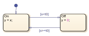
For more information on simulating this chart, see Create Stateflow Charts.
1. Create a Simulink® model called rectify that contains an empty Stateflow Chart block.
sfnew rectify2. Access the Stateflow.Chart object that corresponds to the chart in your model by calling the find function. Use the function sfroot to access the Simulink.Root object, which is the parent of all objects in the Stateflow API.
ch = find(sfroot,"-isa","Stateflow.Chart", ...
    Path="rectify/Chart");
3. Open the chart in the Stateflow Editor by calling the view function.
view(ch);
4. Change the action language by modifying the ActionLanguage property of the chart.
ch.ActionLanguage = "C";Add States
To create a Stateflow API object as the child of a parent object, use the parent object as the input argument to a function that creates the child object. For more information, see Create and Delete Stateflow Objects.
1. Call the Stateflow.State function to add a state to the chart.
s1 = Stateflow.State(ch);
2. Adjust the position of the state by changing the Position property of the corresponding State object. Specify the new position as a four-element vector in which the first two values are the (x,y) coordinates of the upper-left corner of the state and the last two values are the width and height of the state.
s1.Position = [30 30 90 60];
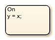
3. Specify the name and label for the state by changing the LabelString property, as described in Specify Labels in States and Transitions Programmatically.
s1.LabelString = "On"+newline+"y = x;";
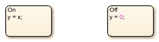
4. Create a second state. Adjust its position and specify its name and label.
s2 = Stateflow.State(ch);
s2.Position = [230 30 90 60];
s2.LabelString = "Off"+newline+"y = 0;";
Add Transitions
When you add a transition, you specify its source and destination by modifying its Source and Destination properties. For a default transition, you specify a destination but no source.
1. Call the Stateflow.Transition function to add a transition to the chart.
t1 = Stateflow.Transition(ch);
2. Set the transition source and destination.
t1.Source = s1;
t1.Destination = s2;
3. Adjust the position of the transition by modifying its SourceOClock property.
t1.SourceOClock = 2.1;
4. Specify the transition label and its position by changing the LabelString and LabelPosition properties.
t1.LabelString = "[x<t0]";
t1.LabelPosition= [159 23 31 16];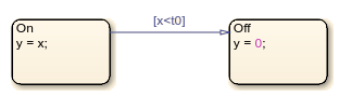
5. Create a second transition. Specify its source, destination, and label.
t2 = Stateflow.Transition(ch);
t2.Source = s2;
t2.Destination = s1;
t2.SourceOClock = 8.1;
t2.LabelString = "[x>=t0]";
t2.LabelPosition= [155 81 38 16];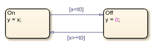
6. Add a default transition to the state On. To make a vertical transition, modify the values of the SourceEndpoint and Midpoint properties. For more information, see Add a Default Transition.
t0 = Stateflow.Transition(ch);
t0.Destination = s1;
t0.DestinationOClock = 0;
t0.SourceEndpoint = t0.DestinationEndpoint-[0 30];
t0.Midpoint = t0.DestinationEndpoint-[0 15];

Add Data
Before you can simulate your chart, you must define each data symbol that you use in the chart and specify its scope and type.
1. Call the Stateflow.Data function to add a data object that represents the input to the chart.
x = Stateflow.Data(ch);
2. Specify the name of the data object as x and its scope as Input.
x.Name = "x";
x.Scope = "Input";
3. To specify that the input x has type double, set its Props.Type.Method property to Built-in. The default built-in data type is double.
x.Props.Type.Method = "Built-in";
x.DataType
ans = 'double'
4. Add a data object that represents the output for the chart. Specify its name as y and its scope as Output.
y = Stateflow.Data(ch);
y.Name = "y";
y.Scope = "Output";
5. To specify that the output y has type single, set its Props.Type.Method property to Built-in and its DataType property to single.
y.Props.Type.Method = "Built-in";
y.DataType = "single";
y.DataType
ans =
'single'
6. Add a data object that represents the transition threshold in the chart. Specify its name as t0 and its scope as Constant. Set its initial value to 0.
t0 = Stateflow.Data(ch);
t0.Name = "t0";
t0.Scope = "Constant";
t0.Props.InitialValue = "0";
7. To specify that the threshold t0 has a fixed-point data type, set its Props.Type.Method property to Fixed-point. Then specify the values of the Props.Type properties that apply to fixed-point data.
t0.Props.Type.Method = "Fixed point";
t0.Props.Type.Signed = true;
t0.Props.Type.WordLength = "5";
t0.Props.Type.Fixpt.ScalingMode = "Binary point";
t0.Props.Type.Fixpt.FractionLength = "2";
t0.DataType
ans =
'fixdt(1,5,2)'
Save and Simulate Your Chart
To save the model that contains your completed chart, call the sfsave function.
sfsave
To simulate the chart, connect it to other blocks in the Simulink model through input and output ports.
1. Add and connect a source to the model:
source = add_block("simulink/Sources/Sine Wave","rectify/Sine Wave");
set_param(source, ...
    SampleTime="0.2", ...
    Position=[-105 30 -75 60]);

sourcePorts = get_param(source,"PortConnectivity");
chartPorts = get_param("rectify/Chart","PortConnectivity");

add_line("rectify",[sourcePorts(1).Position; chartPorts(1).Position]);
2. Add and connect a sink to the model:
sink = add_block("simulink/Sinks/Scope","rectify/Scope");
set_param(sink, ...
    NumInputPorts="2", ...
    Position=[185 21 215 54]);

sinkPorts = get_param(sink,"PortConnectivity");

add_line("rectify", [-25 45; -25 -10; 135 -10; 135 30; 180 30]);
add_line("rectify",[chartPorts(2).Position; sinkPorts(2).Position]);
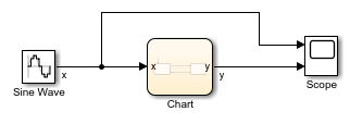
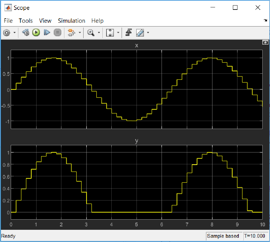
3. Simulate the model.
sim("rectify");4. Double-click the Scope block. The scope displays the graphs of the input and output signals to the charts.