Photovoltaic Thermal (PV/T) Hybrid Solar Panel
This example shows how to model the cogeneration of electrical power and heat using a hybrid PV/T solar panel. The generated heat is transferred to water for household consumption.
It uses blocks from the Simscape™ Foundation™, Simscape Electrical™, and Simscape Fluids™ libraries. The electrical portion of the network contains a Solar Cell block, which models a set of photovoltaic (PV) cells, and a Load subsystem, which models a resistive load. The thermal network models the heat exchange that occurs between the physical components of the PV panel (glass cover, heat exchanger, back cover) and the environment. Heat is exchanged through conduction, convection, and radiation. The thermal-liquid network contains a pipe, a tank, and pumps. The pumps control the flows of the liquids through the system.
To model the reflection, absorption and transmission of light in the glass cover, an optical model is embedded in a MATLAB Function block.
Model Overview
Open the model to view its structure:
open_system('sscv_hybrid_solar_panel');
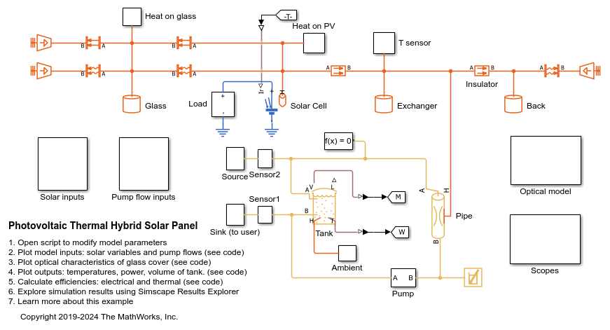
The thermal network is in red, the electrical network in blue and the thermal liquid network in yellow. There are subsystems for the solar and pump inputs. There is also a subsystem that contains scopes for visualizing the simulation results. Another subsystem contains the function for the optical model.
Parameters
You can use the hybrid_solar_panel_data.m script to change the parameter values that this example uses for components such as the load, solar cell, pipe, and tank.
edit sscv_hybrid_solar_panel_data;
Inputs
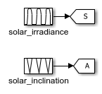
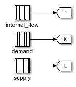
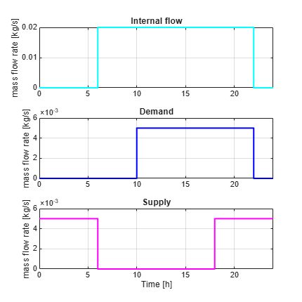
The inputs of the model are the pump flows and the solar variables for irradiance and incidence angle. A repeating sequence block is used to define the inputs because they follow a 24-hour periodic cycle.
open_system('sscv_hybrid_solar_panel/Solar inputs');
open_system('sscv_hybrid_solar_panel/Pump flow inputs');
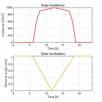
The sun rises at 6:00 and sets at 19:00. The irradiance follows a bell curve that peaks at 12:30. The incidence angle changes from pi/3 to 0.
There are three pumps. One pump models user demand, another models source supply, and a third models internal flow that forces convection in the pipe. The demand is constant and only non-zero from 10:00 to 22:00. The supply is constant and only non-zero from 18:00 to 6:00. The internal flow is also constant and only non-zero from 6:00 to 22:00. This model is used for the internal flow because it is not efficient to force heat exchange during the night when the ambient temperature is low.
You can use the hybrid_solar_panel_plot_inputs.m script to plot the inputs:
sscv_hybrid_solar_panel_plot_inputs;
Optical Model for the Glass Cover
The optical model is inside a subsystem:
open_system('sscv_hybrid_solar_panel/Optical model');
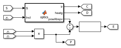
It consists of a MATLAB Function block, with the 2 solar inputs, and 3 outputs: the transmitted irradiance on the PV cells, the heat absorbed by the glass, and the radiative power absorbed by the PV cells. Part of it will be transformed into electrical power (V*I) and the rest will be heat absorbed by the PV cells.
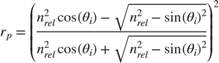
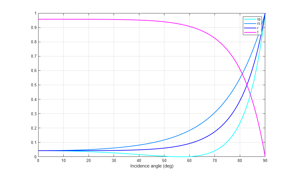
From an optical point of view, the glass consists of 2 parallel boundaries (air-glass, glass-air), each one of those reflects and transmits light. The reflection coefficient in a boundary is obtained from the Fresnel equations.  is for P-polarization and
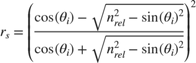
  for S-polarization. The total reflection is the average of both, and the transmittance is
  as there is no absorption so far:


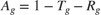
This is an example of the optical coefficients rp, rs, r and t in function of incidence angle:
 nrel = 1.52; %Optical index from air to glass
 theta = linspace(0, pi/2, 100);
 rp = ( nrel^2*cos(theta) - sqrt(nrel^2 - sin(theta).^2) ).^2./...
     ( nrel^2*cos(theta) + sqrt( nrel^2 - sin(theta).^2 ) ).^2 ;
 rs = ( cos(theta) - sqrt(nrel^2 - sin(theta).^2) ).^2./...
     ( cos(theta) + sqrt( nrel^2 - sin(theta).^2 ) ).^2 ;
 r = 0.5*(rp + rs);
 t = 1 - r;

 figure();
 plot(theta*180/pi, rp, 'Color', [0 1 1], 'LineWidth', 1.5);
 hold on
 plot(theta*180/pi, rs, 'Color', [0 0.5 1], 'LineWidth', 1.5);
 plot(theta*180/pi, r, 'Color', [0 0 1], 'LineWidth', 1.5);
 plot(theta*180/pi, t, 'Color', 'm', 'LineWidth', 1.5);
 legend('rp','rs','r','t');
 xlabel('Incidence angle (deg)');
 grid on
 box on
This is what happens in one boundary, but the glass has 2 parallel boundaries separated by  . The angle after the 1st boundary is the incidence angle on the 2nd boundary and is calculated from Snell's Law:
When the light enters the glass, it absorbs part of it with a constant probability per unit length (alpha_g), resulting in an exponential decay from distance travelled for the transmittance coefficient in the glass:
Then, when it arrives at the 2nd boundary, it reflects and transmits again with Fresnel equations. The reflected light is trapped inside the glass, reflecting infinite times between the 2 boundaries until completely absorbed. The total reflection and transmission coefficients of the system are then the sum of an infinite geometrical series, for which the result is:

Finally, the total optical coefficients for the glass are:
sscv_hybrid_solar_panel_plot_optics;
Outputs
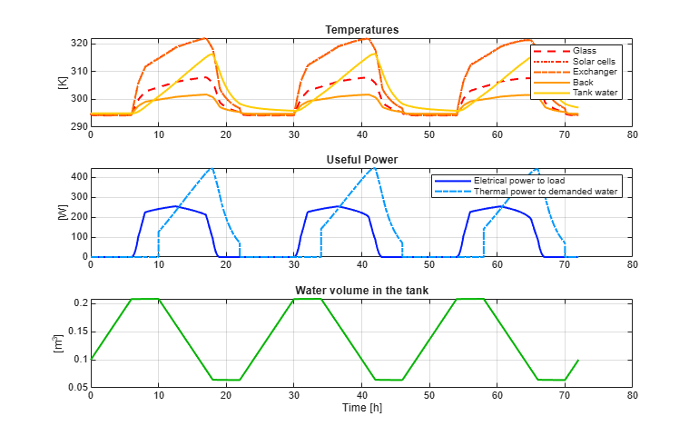
The outputs of the model are the temperatures of all components of the panel, the electrical and thermal power, and the volume in the tank.
You can use the script hybrid_solar_panel_plot_outputs to plot the solution:
sscv_hybrid_solar_panel_plot_outputs;
Efficiency Calculation
From the outputs it is possible to calculate the electrical, thermal, and total efficiency of the panel:
sscv_hybrid_solar_panel_efficiency;
****** Efficiency Calculation *********

Total input energy from the sun in the period: 43.7881 kWh
Average input energy from the sun per day: 14.596 kWh/day

Total electrical energy supplied to the load: 7.5379 kWh
Average electrical energy supplied per day: 2.5126 kWh/day

Total absolute thermal energy in the water supplied to the user: 26.3735 kWh
Total absolute thermal energy in the water extracted from the source: 16.505 kWh

Total used thermal energy (sink - source): 9.8685 kWh
Average used thermal energy per day (sink - source): 3.2895 kWh/day

Electrical efficiency: 0.17215
Thermal efficiency: 0.22537
Total efficiency: 0.39752

***************************************
The electrical efficiency is on the order of standard PV cells, but adding the thermal efficiency the production of energy is significantly better, with a system efficiency on the order of a cogeneration plant.
A further analysis could use Simulink® Design Optimization™ or other optimization tools to find optimal values for certain parameters eligible for control, maximizing total efficiency.
Another improvement would be the addition of controllers to the pumps and the electrical load, in order to drive the system to different operating points and optimize the performance.