Simulate Backplane Channel in Simscape Using S-Parameters

Since R2025a

This example shows how to simulate a differential high-speed backplane channel in Simscape™ using the S-Parameter Rational Fit block. You compare the output of a simulated electrical model for different values of the Rational fit object parameter.

First, you model an ideal channel with no reflections. Then, you calculate block parameter values for a backplane channel using RF Toolbox™. You read a Touchstone® data file that contains single-ended four-port scattering parameters (S-parameters) for a differential high-speed backplane. You convert the four-port S-parameters to two-port differential S-parameters and compute the rational object, which you use as a parameter value in the S-Parameter Rational Fit block. Finally, you simulate the model with the updated parameters and visualize the results.

Open Model

Open the BackplaneChannelSParameters model.

modelName = "BackplaneChannelSParameters";
open_system(modelName)

The Controlled Voltage Source block, labeled Source, supplies a square-wave voltage with an amplitude of 1 V to the electrical network. The S-Parameter Rational Fit block implements a rational approximation of a linear electrical system characterized with S-parameters. In this example, the block represents a high-speed backplane channel that allows power to flow between the source and the Resistor block, labeled Load.

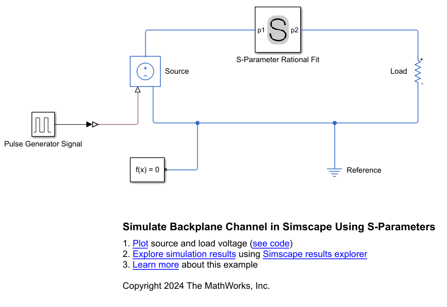
This example shows how to set the S-Parameter Rational Fit block parameters.

Simulate Model with Ideal Channel

Set the Rational fit object to [0 0; 1 0]. With this value, there are no reflections. All power transmits from port p1 to port p2.

set_param(modelName + "/S-Parameter Rational Fit",rfmodelRationalObj = "[0 0; 1 0]")

Simulate the model.

sim(modelName);
idealChannel = simlog;

Plot the voltage across the load and the source for the ideal channel.

plot(idealChannel.Source.v.series.time,idealChannel.Load.v.series.values,"-",idealChannel.Source.v.series.time,idealChannel.Source.v.series.values,"--")
ylim([-0.2,1.2]);
legend("Load","Source")
title("Ideal Channel")
xlabel("Time (s)")
ylabel("Voltage (V)")

The plot shows that the voltage profiles overlap because the ideal channel allows all the power from the source to flow to the load.

Simulate Model with Backplane Channel

Now, simulate the model with a high-speed backplane channel using the Touchstone data.

First, read the default.s4p Touchstone data file into an sparameters (RF Toolbox) object. The data file contains the 50 Ohm S-parameters of a single-ended four-port passive circuit, measured at 1496 frequencies ranging from 50 MHz to 15 GHz.

filename = "default.s4p";
backplane = sparameters(filename);

Get the single-ended four-port S-parameters from the backplane data object.

data = backplane.Parameters;
freq = backplane.Frequencies;
z0 = backplane.Impedance;

Convert the data to two-port differential S-parameters using the s2sdd (RF Toolbox) command.

diffdata = s2sdd(data,1); 

Fit a rational function object to the data over the specified frequencies using the rational (RF Toolbox) function.

rationalFunction = rational(freq,diffdata,NumPoles = 100);

Set the Rational fit object parameter of the S-Parameter Rational Fit block to rationalFunction.

set_param(modelName + "/S-Parameter Rational Fit", rfmodelRationalObj = "rationalFunction")

Simulate the model.

sim(modelName);
backplaneChannel = simlog;

Plot the voltage across the load and the source for the backplane channel.

plot(backplaneChannel.Source.v.series.time,backplaneChannel.Load.v.series.values,"-",backplaneChannel.Source.v.series.time,backplaneChannel.Source.v.series.values,"--")
ylim([-0.2,1.2])
legend("Load","Source")
title("Backplane Channel")
xlabel("Time (s)")
ylabel("Voltage (V)")

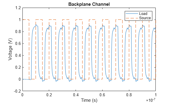
When the model includes the backplane channel some of the power from the source reflects. Power losses reduce the peak voltage across the load compared to the idealized case and introduce a delay relative to the source. Reflections in the S-Parameter Rational Fit block reduce the minimum voltage across the load to below zero.

Close Model

Close the model.

close all
close_system(modelName,0)