Discrete-Valued Variables in Response Optimization (GUI)
This example shows how to use response optimization to tune discrete-values variables. Discrete-valued variables represent model parameters that are restricted to a finite set of values, instead of continuously varying. To use discrete-values variables for response optimization or parameter estimation, you must use the Surrogate optimizer for mixed-integer optimization. For a similar optimization performed at the command line, see Discrete-Valued Variables in Response Optimization (Code).
Open the Model
In the sdoMotorPosition model, a PI controller enables the angular position of a DC motor to match a desired reference value. The load on the motor is subject to disturbances, and the controller must reject these disturbances.
open_system('sdoMotorPosition');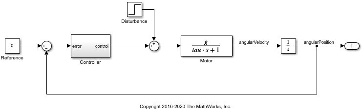
Within the Controller subsystem, the PI gains are set by a 12 V source divided down by resistors R1, R2, R3, and R4, as shown in the following diagram.

The proportional gain, Kp, is given by 12*R2/(R1+R2) and the integral gain, Ki, is given by 12*R4/(R3+R4). The initial values of the resistances are R1 = 47 kΩ, R2 = 180 kΩ, R3 = 10 kΩ, and R4 = 10 kΩ.
Open the Response Optimizer App
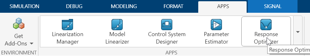
In the Simulink® toolstrip, select Response Optimizer.
Specify Design Variables
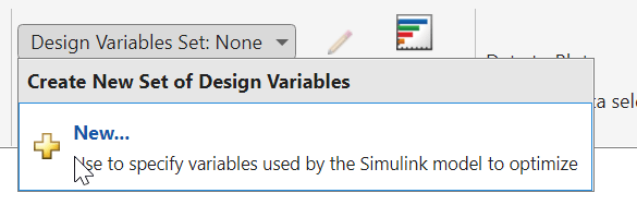
The four resistor values R1, R2, R3, and R4 are the model parameters to tune for the optimization. Because resistors are only available in discrete values, you can use discrete parameters to represent them, specifying the values they are allowed to take on. To make these specifications in the app, start by adding a new set of design variables. Click Design Variables Set: None and select New.
This action opens the Create Design Variables Set dialog box. The right hand side is already populated with all the candidate variables in the Simulink model. To specify the resistor value R1 as a discrete variable, select it, and click ![]() .
.
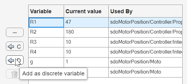
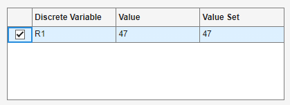
The variable R1 appears in the Discrete Variable table on the lower left of the dialog box.
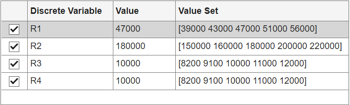
Repeat this procedure to add R2, R3, and R4 as discrete parameters. The Value Set column contains the values that the discrete parameters can take during the optimization. Initially, the app uses the current value of the parameter to populate this column. Modify the Value Set column to set the following allowed values for the four resistors.
R1: [39000 43000 47000 51000 56000]R2: [150000 160000 180000 200000 220000]R3: [8200 9100 10000 11000 12000]R4: [8200 9100 10000 11000 12000]
Finally, click OK to save the design variables set and close the dialog box.
Specify Signals and Design Requirements
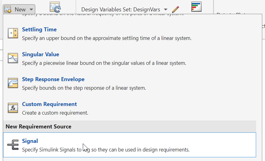
The model applies a step disturbance at 1 second. With the initial resistance values specified in the model, the disturbance causes the motor to deviate by about 20°. The response then settles back to within ±5° of the reference position by 4 seconds after the disturbance. For this example, find new resistor values to improve this specification by 10%, so that the motor deviates no more than 18°, and settles back to within ±4.5° degrees of the reference position by 4 seconds after the disturbance. First, specify the motor response signal as the source for the design requirement. To do so, in the app, click ![]() New. Scroll down to the New Requirement Source section and select Signal.
New. Scroll down to the New Requirement Source section and select Signal.
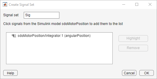
Next, in the model canvas, select the angular position signal.

This action adds the signal to the signal set in the Create Signal Set dialog box.
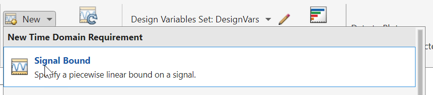
Click OK to save this signal set. Now, add signal bound requirements to capture the target response as upper and lower bounds on this signal. To do so, click ![]() New again and select Signal Bound.
New again and select Signal Bound.
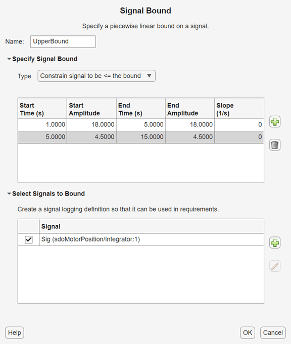
In the Create Requirement dialog box, in the Name field, enter UpperBound to name the signal-bound requirement. Then, specify the appropriate amplitude and time bounds for the upper bound. First, set the initial upper bound on the motor deflection of no more than 18°. Then click ![]() to add second upper bound, ensuring that the signal settles to no more than 4.5° above the reference position by 4 seconds after the disturbance. Finally, select the signal set you created earlier to apply these upper bound to that signal.
to add second upper bound, ensuring that the signal settles to no more than 4.5° above the reference position by 4 seconds after the disturbance. Finally, select the signal set you created earlier to apply these upper bound to that signal.
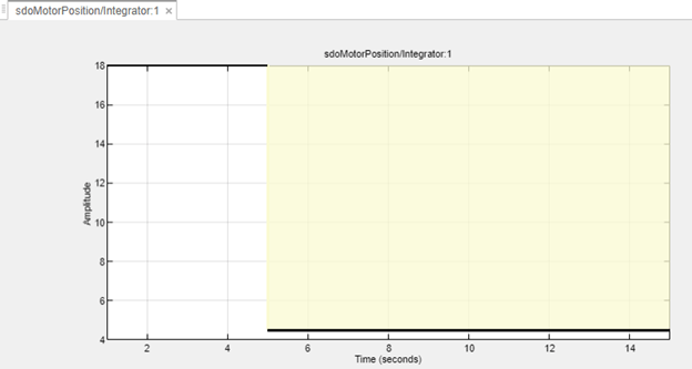
Click OK to save the requirement. The app displays the bounds graphically so that you can verify that you have entered them correctly.
Similarly, create another signal bound to specify the lower bounds on the signal. This time, in the Type drop-down menu, select Constrain signal to be >= the bound to create a lower bound. For the lower bound, ensure that the final deflection is no more than 4.5° below the reference position. Click OK to save this bound.

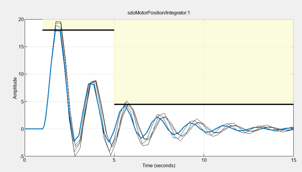
To visualize the initial response of the model, click Plot Model Response.
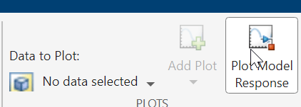
This action simulates the model and plots the specified signals on the bounds. The bounds are shown in black, while the motor position is shown in blue. The response with the initial resistance values does not quite satisfy the bounds.

Set up Optimization
The optimization process runs the model many times with different values for the resistor variables. To expedite this process, configure the simulator for fast restart. In the Simulink model canvas, in the Modeling tab, select Fast Restart.

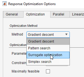
Optimizations using discrete parameters require the surrogate optimization method. In the Response Optimizer app, click Options and select Optimization. Then, in the Response Optimization Options dialog box, in the Optimization tab, in the Method drop-down menu, select Surrogate optimization.
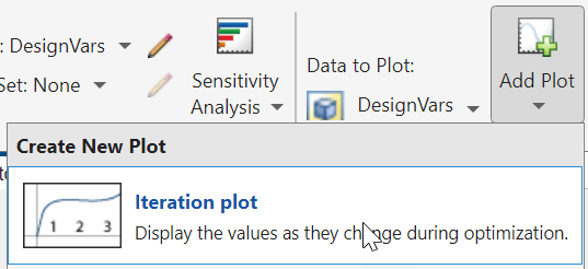
Finally, to visualize the design variables during optimization, add a parameter iteration plot. In the app, under Data to Plot, click No data selected and select DesignVars, the set of design variables you created earlier with the four resistor values. Then, click Add Plot and select Iteration plot. This action creates a plot that displays the values of the design variables as each iteration completes.
Optimize the Design
To start the optimizer, in the Response Optimization tab, click ![]() Optimize. The model runs once for each iteration, updating the requirement and parameter iteration plots. When the specified number of iterations for surrogate optimization is reached, the optimization stops. When the optimization ends, the app automatically updates the model parameters with the optimized values.
Optimize. The model runs once for each iteration, updating the requirement and parameter iteration plots. When the specified number of iterations for surrogate optimization is reached, the optimization stops. When the optimization ends, the app automatically updates the model parameters with the optimized values.

Evaluate Optimized Design
The requirement plot for the upper bound shows that the motor position signal does not breach the chosen limits any more.
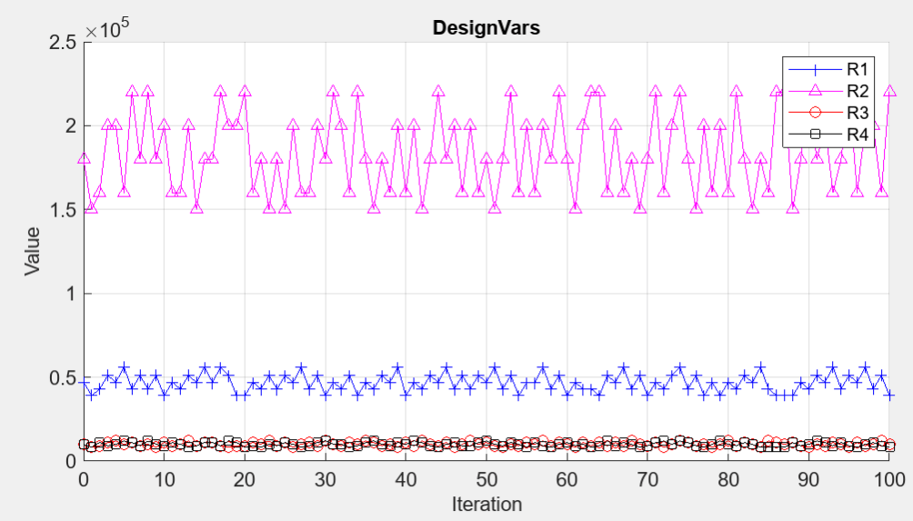
The parameter iteration plot shows how the Surrogate optimizer explores the design space.
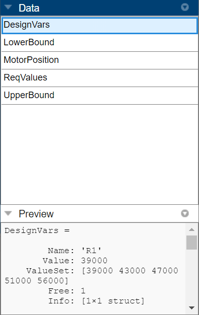
You can view the optimized design variable values in the preview pane of the browser.
Conclusion
In this example you tuned variables to improve the disturbance rejection characteristics of a motor controller. The variables being tuned were electrical component parts that could only take on discrete values, rather than continuous values. You used the Response Optimizer app and the Surrogate optimizer to tune the parameters.
See Also
sdo.optimize | param.Discrete | sdo.getParameterFromModel | sdo.OptimizeOptions