Tune PID Controller for Mass-Spring-Damper System Using VRFT at Command Line

Since R2026a

This example shows how to use the VRFT command-line API to tune a PID controller for a mass-spring-damper system. The input-output data is extracted directly from the simulation results of a Simulink® model.

Mass-Spring-Damper Plant Model

The mass-spring-damper system consists of two carts with masses $m_1$ and $m_2$, connected to each other and to the ground by springs and dampers. The springs have stiffness coefficients $k_1$and $k_2$, and the dampers have damping coefficients $c_1$ and $c_2$.

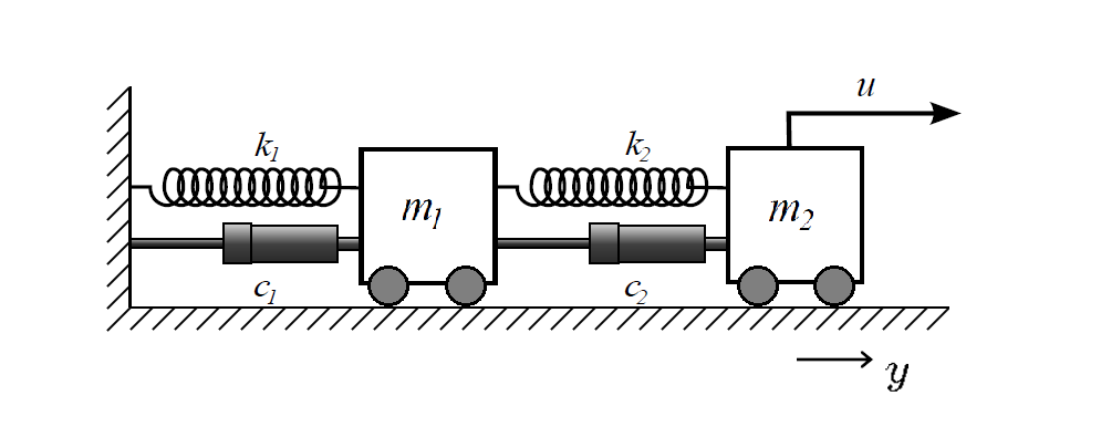
Define the parameters.

m1 = 1;
m2 = 0.5;
c1 = 0.2;
c2 = 0.5;
k1 = 1;
k2 = 0.5;

Define an LTI plant model for the mass-spring-damper system based on the given parameters.

sys_tf = tf([m1 c1+c2 k1+k2],[m1*m2 m2*(c1+c2)+m1*c2 m2*(k1+k2)+m1*k2+c1*c2 c1*k2+k1*c2 k1*k2])

sys_tf =
 
               s^2 + 0.7 s + 1.5
  -------------------------------------------
  0.5 s^4 + 0.85 s^3 + 1.35 s^2 + 0.6 s + 0.5
 
Continuous-time transfer function.
Model Properties

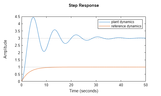
As part of the VRFT settings, the reference model defines the desired closed-loop behavior for the tuned PID controllers. In this example, the reference model is a continuous-time first-order system represented by the transfer function tf(1,[3 1]). The following plot compares the step responses of the open-loop plant and the desired closed-loop behavior.

figure;
step(sys_tf,tf(1,[3 1]))
legend('plant dynamics','reference dynamics')

Log Data from Closed-Loop Simulink Model

Open the Simulink® model that includes an LTI plant object. This model contains an initial PID controller that regulates the output and a Virtual Reference Feedback Tuning block to tune the PID parameters so the closed-loop response closely matches the reference system tf(1,[3 1]). After tuning, you compare the PID gains obtained in Simulink with those computed at the command line.

mdl = 'TuningOfPIDControllerUsingVRFTAPI.slx';

Simulate the model to log data. Extract the full input and output from the Simulink.SimulationData.Dataset object.

Ts = 0.1;
SimOut = sim(mdl);
TT = extractTimetable(SimOut.ScopeData);

Prepare Logged Data for Tuning

The tuning interval in the Simulink® model is from 1 s to 400 s, and the sample time is 0.1 s.

Ts = 0.1;
t = 1:Ts:400;
TT_simulink = retime(TT,seconds(t),'nearest');

Provide Reference Model and Weight Function

Provide a reference model as an LTI object to define the desired closed-loop performance. Optionally, provide a weighting function as an LTI object to emphasize specific frequency ranges. If the LTI objects are continuous-time, vrfttune discretizes them during tuning.

MrefS = tf(1,[3 1]);
WeightS = tf(1,[0.3 1]);

Define Controller Structure

This example uses the "parallel-pid" option to define the PID controller for tuning.

optionsParallelPID = vrfttuneOptions('parallel-pid');
optionsParallelPID.PIDType = 'PID';
optionsParallelPID.IntegratorMethod = 'Trapezoidal';
optionsParallelPID

optionsParallelPID = 
  ParallelPID with properties:

                 PIDType: 'PID'
        IntegratorMethod: 'Trapezoidal'
    DiscretizationMethod: 'tustin'

Tune PID Controller Parameters

To tune the PID controller parameters, use the vrfttune function.

[thetaParam_parallel_pid,tunedblk_parallel_pid,info_parallel_pid]...
    = vrfttune(TT_simulink,MrefS,WeightingFunction = WeightS,VRFTOptions=optionsParallelPID);

Compare the tuned PID controller parameters from vrfttune with the tuning results from the Simulink model using the Virtual Reference Feedback Tuning block.

thetaParam_simulink = SimOut.theta.signals.values';
T = table(thetaParam_simulink, thetaParam_parallel_pid);
T.Properties.RowNames = {'Kp','Ki','Kd'}

T=3×2 table
          thetaParam_simulink    thetaParam_parallel_pid
          ___________________    _______________________

    Kp         0.062357                 0.062355        
    Ki          0.11191                  0.11191        
    Kd          0.22526                  0.22526        

As demonstrated, you can directly convert logged data from a Simulink model into a timetable object. This enables a smooth offline VRFT workflow for tuning linear controllers. The tuning results are consistent with those obtained using the VRFT block.