Soft Robot Control Using Iterative Learning Control

Since R2026a

This example demonstrates control of soft robot using the Iterative Learning Control (ILC) block in Simulink®. The soft-robot arm is commanded to track a step signal, while the actuators are pressure actuated using soft bellows. This example demonstrates, using ILC over repeated iterations, the controller learns to minimize error and get close tracking of given reference signal.

Soft-Robot Model

In this example we will demonstrate the soft-robot control using PID augmented by ILC controller. The hybrid soft-robotic arm considered in the example consists of two soft actuators and a rigid link with an arm as shown in the figure below. The differential pressure in the two bellows actuates the arm in either direction [1].

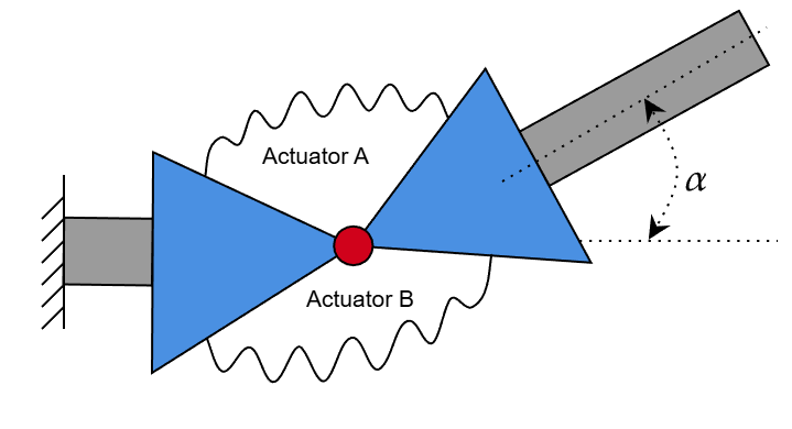
Before we introduce a 1-DOF model, lets introduce few variables

• $k$ denotes time index

• $\left(x_1,x_2\right)=\left(\alpha ,\underset{}{\overset{\dot{}}{\alpha }}\right)$ are the angle and angular velocity of the arm

• $\Delta p=p_A-p_B$is the differential pressure, the control input $u\left(k\right)$.

• $p_A,p_B$ are the soft actuator bellow pressures.

This example use a simplified linear time-invariant dynamic model [1] as follows,

$$\begin{array}{l}\left[\begin{array}{c}{x}_1\left(k\right)\\ x_2\left(k\right)\end{array}\right]=\left[\begin{array}{cc}0.96& 0.18\\ -0.36& 0.80\end{array}\right]\left[\begin{array}{c}{x}_1\left(k-1\right)\\ x_2\left(k-1\right)\end{array}\right]+\left[\begin{array}{c}0.09\\ 0.91\end{array}\right]u\left(k-1\right)\\ y\left(k\right)=\left[\begin{array}{cc}1& 0\end{array}\right]\left[\begin{array}{c}{x}_1\left(k\right)\\ x_2\left(k\right)\end{array}\right]\end{array}$$

The arm deflection $\alpha$ is directly measured using a rotary encoder.

The discretized system use the sample time Ts = 1/50s

% Sample Time
Ts = 1/50;

Cascaded controller for soft-robot arm

A cascaded control architecture is applied to soft-robotic arm based on the time scale separation. The two time scales are the faster pressure dynamics in the inner loop and the slower arm dynamics in the outer loop.

A proportional-integral-derivative (PID) controller is used in the outer loop to compute the required pressure difference to reach the desired angle of the arm. The baseline PID controller $u_{\text{pid}}$ designed to do the angle tracking such that $y\to y_d$, where $y_d$ is the desired angle.

$$u_{\text{pid}}=k_{p_{}}\left(y_d-y\left(k\right)\right)+k_{d_{}}\left(\underset{}{\overset{\dot{}}{y_d}}-\underset{}{\overset{\dot{}}{y}}\left(k\right)\right)+k_{I_{}}\int \left(y_d-y\left(k\right)\right)\text{dt}$$

The individual desired set points pressure for the inner loop can be computed from set point for pressure difference computed using ${\Delta p^{*}=u}_{\text{pid}}$as follows,

$p_A^{*}=\min \left(p_{\max },\max \left(p_{0,}{p}_0+u_{\text{pid}}\right)\right)$,

$p_B^{*}=\min \left(p_{\max },\max \left(p_{0,}{p}_0-u_{\text{pid}}\right)\right)$,

where $p_0=1\text{bar}$ is the ambient air pressure and $p_{\max }=1.4\text{bar}$ is maximum allowed pressure.

% Define ambient and max pressure for the actuators
p0 = 1;
pmax = 1.4;

Consider a first-order actuator dynamics in the inner loop for the pressure bellows as follows.

$\underset{}{\overset{\dot{}}{p_A}}=\frac{1}{{\tau }_p}\left(p_A^{*}-p_A\right)$,

$$\underset{}{\overset{\dot{}}{p_B}}=\frac{1}{{\tau }_p}\left(p_B^{*}-p_B\right)$$

where ${\tau }_p$ is the time constant for the pressure actuator dynamics. In this example you will use same time constant as plant

% Actuator time constant
tau_p = 1/Ts;

Outer Loop position control for soft-robotic arm

The outer loop, PID control tracks the desired angle for the robotic arm an inner loop tracks the desired actuator pressure. The cascaded outer-inner loop dynamics for soft-robotic arm is as follows.

This example use a PI controller in the outer loop. The tuned baseline PI controller gains are as follows,

% Outer-Loop PID gain
Kp = 0.001;
Ki = 0.3;

Iterative learning Control Overview

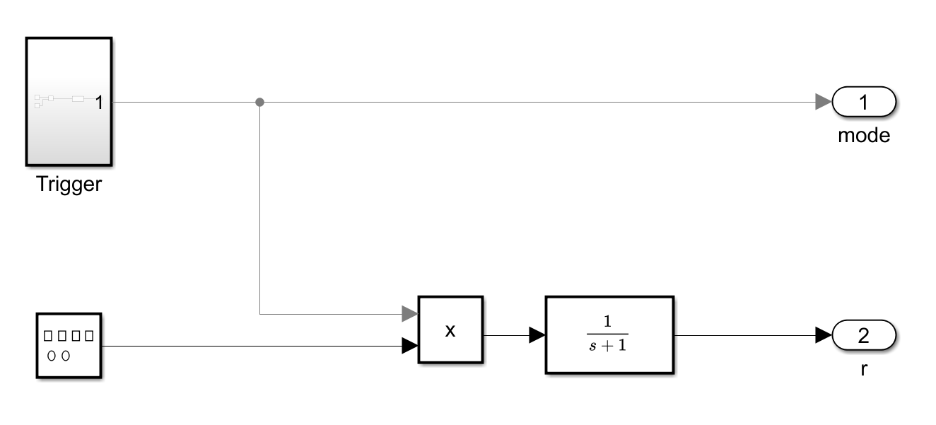
The outer-loop control of the arm angle is augmented with ILC control as shown in figure below. The soft-robotic arms repeatedly track the step signal $\left(-\frac{\pi }{6},\frac{\pi }{6}\right)$for N iterations. The ILC controller aim is, over the iterations gradually improve tracking performance.

Iterative learning control (ILC) is an improvement in run-to-run control. It uses frequent measurements in the form of the error trajectory from the previous batch to update the control signal for the subsequent batch run. The focus of ILC has been on improving the performance of systems that execute a single, repeated operation, starting at the same initial operating condition. This focus includes many practical industrial systems in manufacturing, robotics, and chemical processing, where mass production on an assembly line entails repetition.

• Suitable for repetitive task + repetitive disturbances.

• Use knowledge from previous iteration to improve next iteration.

A general ILC control update is as follows [2],

$$u_{n+1}\left(k\right)=Q\left(q\right)\left[u_n\left(k\right)+L\left(q\right)e_n\left(k+1\right)\right]$$

Where L is learning function. In this example, you compare model-free vs model based (Inverse-model) ILC.

• Model free ILC: The learning function $L=\left({\gamma }_p,{\gamma }_d\right)$ are the fixed gains.

• Inverse-Model ILC use learning function $L=G^{-1}$, where G is the input-output relation for LTI system, in the lifted form such that $y_n={\text{Gu}}_n+d$.

For more details, see Iterative Learning Control.

ILC mode

At runtime, ILC switches between two modes: control and reset. In the control mode, ILC outputs $u_n\left(k\right)$at the desired time points and measures the error between the desired reference $y_d\left(k\right)$ and output $y_n\left(k\right)$. At the end of the control mode, ILC calculates the new control sequence $u_{n+1}\left(k\right)$ to use in the next iteration. In the reset mode, ILC output is 0. The reset mode must be long enough for return to home controller to bring the plant back to its initial condition.

Model-Free ILC Design

To design model-free ILC controller, following parameters are required to be configured,

• Sample time and Iteration duration — These parameters determine how many control actions ILC provides in the control mode.

• ILC gains $\left({\gamma }_p,{\gamma }_d\right)$ — ILC gains update the ILC control based error feedback.

• Filter time constant — The optional low-pass filter to remove control chatter which may otherwise be amplified during learning. By default it is not enabled in the ILC block.

Configure the example model to Model-free ILC model.

mdl = 'SoftRobotILC';
open_system(mdl)

% Switch to model free ILC
set_param([mdl, '/ILC'], 'Algorithm', 'Model free ILC')

Lets define the parameters for the ILC block.

% single iteration duration
Tspan = 20;

The proportional and derivative ILC gain ${\gamma }_p,{\gamma }_d$ are selected as follows,

% ILC gain
gamma_p = 2;
gamma_d = 15;

ILC implements a low pass filter to filter out high-gain control oscillations. Filter adds trade-off between rate of convergence and robustness.

% Filter Coeff
Filter_coeff = 50;

% Enable the filter
set_param([mdl, '/ILC'], 'LPFenable', 'on')

Simulate Model and Plot Results

Simulate the model for 20 iterations. In the first iteration, ILC controller outputs "0" in the control mode. Therefore, the closed-loop control performance displayed in the first iteration comes from the nominal controller, which serves as the baseline for the comparison.

% Simulate the model
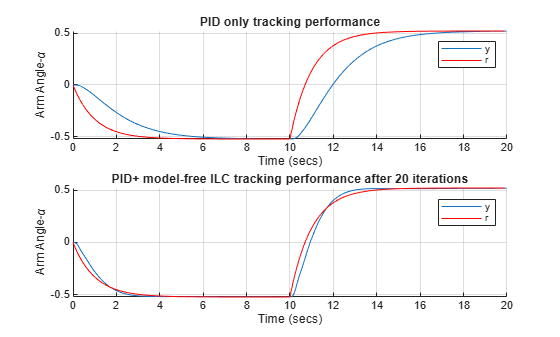
simout = sim(mdl);

As the iterations progress, the ILC controller improves the reference tracking. Comparing the PID tracking to the improved tracking performance after applying ILC for 20 iterations

% Plot Soft-robot tracking performance PID vs PID+ILC
figure(2)
tiledlayout(2,1,TileSpacing="tight");
nexttile
hold on
grid on
yk = squeeze(simout.y.Data);
plot(simout.y.Time(1:1000), yk(1:1000))
plot(simout.r.Time(1:1000), simout.r.Data(1:1000),'Color','r')
xlabel('Time (secs)')
ylabel('Arm Angle-\alpha')
title('PID only tracking performance')
legend('y','r')

nexttile
hold on
grid on
yk = squeeze(simout.y.Data);
plot(simout.y.Time(1:1000), yk(end-2000:end-1001))
plot(simout.r.Time(1:1000), simout.r.Data(1:1000),'Color','r')
xlabel('Time (secs)')
ylabel('Arm Angle-\alpha')
title('PID+ model-free ILC tracking performance after 20 iterations')
legend('y','r')

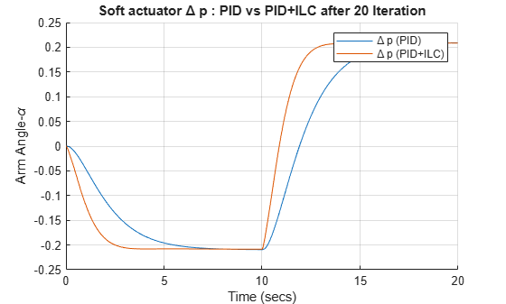
Actuator $\Delta p=p_A-p_B$ for PID and PID + ILC after 20 iterations,

% Soft Actuator pressure PID vs PID+ILC
figure(3)
hold on
grid on
delta_p = squeeze(simout.deltap.Data);
plot(simout.y.Time(1:1000), delta_p(1:1000))
plot(simout.y.Time(1:1000), delta_p(end-2000:end-1001))
xlabel('Time (secs)')
ylabel('Arm Angle-\alpha')
title('Soft actuator \Delta p : PID vs PID+ILC after 20 Iteration')
legend('\Delta p (PID)','\Delta p (PID+ILC)')

Plot the control effort in the outer loop PID+ILC controller

figure(4)
tiledlayout(2,1,TileSpacing="tight");
% Plot ILC control
nexttile
plot(squeeze(simout.uilc.Data))
xlabel('Time')
ylabel('u');
title('ILC Control')
% Plot PID control
nexttile
plot(squeeze(simout.upid.data))
xlabel('Time')
ylabel('u');
title('PID Control')

Model-based ILC Design

To design model-based ILC controller, following parameters are required to be configured,

• Sample time and Iteration duration — These parameters determine how many control actions ILC provides in the control mode.

• Model information --- This example use model based ILC. A nominal closed loop model information is necessary to design the ILC controller.

• ILC gains — The gain determine how quick ILC learns between iterations. If ILC gain is too big, it might make the closed-loop system unstable (robustness). If ILC gains are too small, it might lead to slower convergence (performance).

• Filter time constant — The optional low-pass filter to remove control chatter which may otherwise be amplified during learning. By default it is not enabled in the ILC block.

Configure the example model to Model-based ILC model

mdl = 'SoftRobotILC';

% Switch to model based ILC
set_param([mdl, '/ILC'], 'Algorithm', 'Model based ILC')

For a model based version of ILC you will require a nominal linear discrete model for the system.

% Nominal plant for ILC
Ap = '[0.96 0.18;-0.36 0.80]';
Bp = '[0;0.91]';
Cp = '[1 0]';

% Set the nominal plant parameters for ILC
set_param([mdl, '/ILC'], 'A', Ap, 'B', Bp, 'C', Cp);

ILC gain for model inverse ILC is selected as follows, this gain control learning rate for ILC updates

% ILC gain
gamma_inverse = '1.25';
set_param([mdl, '/ILC'], 'gamma_inverse', gamma_inverse)

For model based ILC, do not implement an output filter.

% Disable the filter
set_param([mdl, '/ILC'], 'LPFenable', 'off')

Simulate Model and Plot Results

Similar to model-free, simulate the controller for 20 iterations.

% Simulate the model
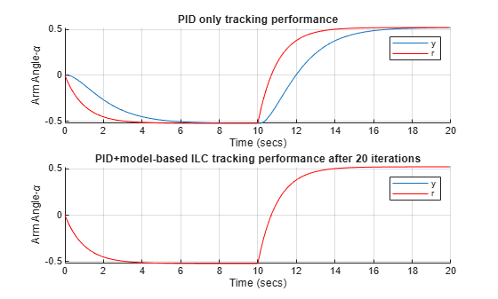
simout = sim(mdl);

As the iterations progress, the ILC controller improves the reference tracking. Comparing the PID tracking to the improved tracking performance after applying ILC for 20 iterations

% Plot Soft-robot tracking performance PID vs PID+ILC
figure(6)
tiledlayout(2,1,TileSpacing="tight");
nexttile
hold on
grid on
yk = squeeze(simout.y.Data);
plot(simout.y.Time(1:1000), yk(1:1000))
plot(simout.r.Time(1:1000), simout.r.Data(1:1000),'Color','r')
xlabel('Time (secs)')
ylabel('Arm Angle-\alpha')
title('PID only tracking performance')
legend('y','r')

nexttile
hold on
grid on
yk = squeeze(simout.y.Data);
plot(simout.y.Time(1:1000), yk(end-2000:end-1001))
plot(simout.r.Time(1:1000), simout.r.Data(1:1000),'Color','r')
xlabel('Time (secs)')
ylabel('Arm Angle-\alpha')
title('PID+model-based ILC tracking performance after 20 iterations')
legend('y','r')

Actuator $\Delta p=p_A-p_B$ for PID and PID + ILC after 20 iterations,

% Soft Actuator pressure PID vs PID+ILC
figure(7)
hold on
grid on
delta_p = squeeze(simout.deltap.Data);
plot(simout.y.Time(1:1000), delta_p(1:1000))
plot(simout.y.Time(1:1000), delta_p(end-2000:end-1001))
xlabel('Time (secs)')
ylabel('Arm Angle-\alpha')
title('Soft actuator \Delta p : PID vs PID+ILC after 20 Iteration')
legend('\Delta p (PID)','\Delta p (PID+ILC)')

Plot the control effort in the outer loop PID+ILC controller

figure(8)
tiledlayout(2,1,TileSpacing="tight");
% Plot ILC control for X Direction
nexttile
plot(squeeze(simout.uilc.Data))
xlabel('Time')
ylabel('u');
title('ILC Control')
% Plot PID control for X Direction
nexttile
plot(squeeze(simout.upid.data))
xlabel('Time')
ylabel('u');
title('PID Control')

As iterations progress the ILC controller learns to compensate for the tracking error and the nominal PID control effort is reduced to a minimum.

Conclusion

In this example, you designed an Iterative learning controller for soft-robot. This example compared model-free vs model-based ILC. Both ILC controllers were successful in achieving better tracking compared to baseline PI. As expected, model-based ILC provide better tracking performance compared to model-free ILC, but requires additional model information for controller design.

% Close the model
close_system(mdl,0);

References

1. Hofer, Matthias, Lukas Spannagl, and Raffaello D’Andrea. "Iterative learning control for fast and accurate position tracking with an articulated soft robotic arm." 2019 IEEE/RSJ International Conference on Intelligent Robots and Systems (IROS). IEEE, 2019.

2. Bristow, Douglas A., Marina Tharayil, and Andrew G. Alleyne. “A Survey of Iterative Learning Control.” IEEE Control Systems 26, no. 3 (June 2006): 96–114.