Design Active Disturbance Rejection Control for Water-Tank System
This example shows how to design active disturbance rejection control (ADRC) for a nonlinear water-tank system.
Water-Tank System Model
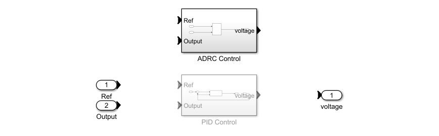
This model uses an ADRC controller to control the water level of a nonlinear Water-Tank System plant. The model contains a variant subsystem with two choices: an ADRC controller and a gain-scheduled PID controller. The ADRC Control subsystem is set as the default active variant. The model also includes a manual switch to operate the model in open-loop and closed-loop configurations. It is set to an open-loop configuration by default.
Although a gain-scheduled PID controller is an effective way to control the plant output over a wide operating range, designing experiments and tuning PID gains using the Closed-Loop PID Autotuner require significant efforts. Using ADRC you can obtain a nonlinear controller and achieve better performance with a simpler setup and less tuning effort. For more information on how to tune a gain-scheduled PID controller, see Tune Gain-Scheduled Controller Using Closed-Loop PID Autotuner Block.
Open the model.
mdl = 'WatertankADRC';
open_system(mdl)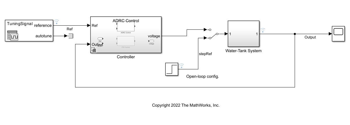
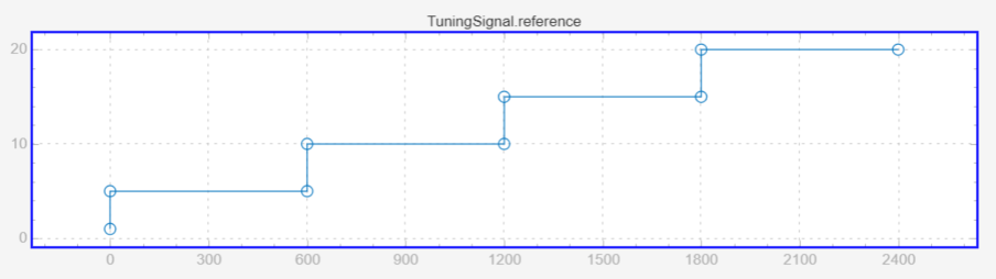
The water-level reference signal in this example is the same as the reference signal in the gain-scheduled controller autotuning example. The reference water level rises gradually from = 1 to four operating points at = [5, 10, 15, 20]. Each step of water-level change takes 600 seconds.
Design ADRC Controller
ADRC is a powerful tool for the controller design of a plant with unknown dynamics and internal and external disturbances. The block models unknown dynamics and disturbances as an extended state of the plant and estimates them using an observer. The ADRC block lets you design a controller using only a few key tuning parameters for the control algorithm:
Model order type (first-order or second order)
Critical gain of the model response
Controller and observer bandwidths
Additionally, specify the Time domain parameter to match the time domain of the plant model. In this example, set it to continuous-time. The following sections describe how to find the remaining tuning parameters specified in the ADRC block parameters for this model.
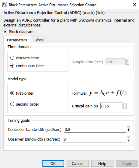
Model Order and Critical Gain
For this water-tank model, it is easy to tune these parameters. Inject a step input with amplitude 1 into the Water-Tank System subsystem and note that the open-loop water-level response shows a first-order dynamic system behavior.
sim(mdl);
figure;
plot(logsout{2}.Values.Time,logsout{2}.Values.Data...
    ,logsout{3}.Values.Time,logsout{3}.Values.Data)
grid on
ylim([0 7])
xlabel('Time (s)')
ylabel('Height (m)')
legend('Ref','Output')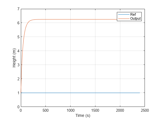
To determine the critical gain value b0, examine the water-level response over a short interval of 0.5 seconds right after the step reference input.
x = logsout{3}.Values.Time(1:57);
y = logsout{3}.Values.Data(1:57);
figure;
plot(x,y)
xlabel('Time (s)')
ylabel('Height (m)')
grid on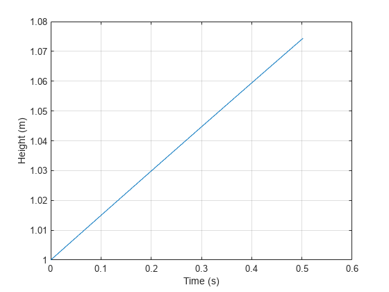
You can now determine the critical gain for the system based on the first-order response . Over a duration of 0.5 seconds, the water-level increases by around 0.075 m.
Find Controller Bandwidth and Observer Bandwidth
The controller bandwidth usually depends on the performance specifications, either in the frequency domain or time domain. This example uses a relaxed controller bandwidth of 0.8 rad/s. The observer needs to converge faster than the controller, so the observer bandwidth is typically set to 5 to 10 times the controller bandwidth. As an initial tuning attempt, you can choose rad/s.
Toggle the manual switch to operate the model in the closed-loop configuration.
set_param('WatertankADRC/Manual Switch','sw','1')
Simulate the model to examine the water level corresponding to a step reference change, such as from 15 to 20.
set_param(mdl,'SignalLoggingName','adrcOut');
sim(mdl);
figure
plot(adrcOut{1}.Values.Time,adrcOut{1}.Values.Data...
    ,adrcOut{3}.Values.Time,adrcOut{3}.Values.Data)
grid on
ylim([14 21])
xlim([1700 1950])
xlabel('Time (s)')
ylabel('Height (m)')
legend('Ref','Output')
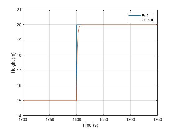
Based on the response, you can see that the water-level response is fast enough, and the overshoot is minimal. As a result, the ADRC block setup and parameter tuning is complete.
Performance Comparison of ADRC and PID Controller
Examine the tuned controller performance using the water-level reference signal with multiple operating points.
Select the PID Control subsystem and simulate the model.
set_param([mdl,'/Controller'],'LabelModeActiveChoice','PID')
set_param(mdl,'SignalLoggingName','pidOut');
sim(mdl);
Compare the performance of the two controllers.
figure;
plot(adrcOut{1}.Values.Time,adrcOut{1}.Values.Data...
    ,adrcOut{3}.Values.Time,adrcOut{3}.Values.Data)
hold on
plot(pidOut{3}.Values.Time,pidOut{3}.Values.Data)
hold off
grid on
xlabel('Time (s)')
ylabel('Height (m)')
legend('Ref','ADRC','PID')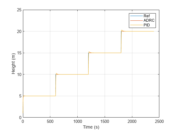
The water-level response shows that the ADRC controller performs much better than the gain-scheduled PID controller and follows the water-level reference signal more closely with much less overshoot.
You can further zoom into when the water level response increases from 15 to 20 to see the improved performance.
figure;
plot(adrcOut{1}.Values.Time,adrcOut{1}.Values.Data...
    ,adrcOut{3}.Values.Time,adrcOut{3}.Values.Data)
hold on
plot(pidOut{3}.Values.Time,pidOut{3}.Values.Data)
hold off
grid on
xlabel('Time (s)')
ylabel('Height (m)')
legend('Ref','ADRC','PID')
ylim([14 21])
xlim([1700 1950])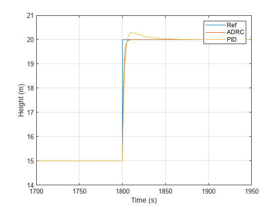
Close the model.
close_system(mdl,0);
See Also
Active Disturbance Rejection Control