Model Oscillation Sensor Using Permanent Magnet Block

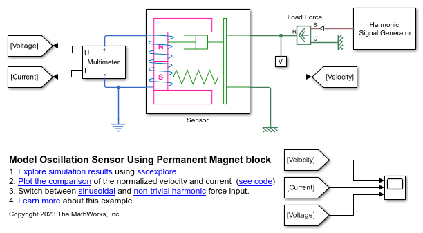
This example shows how to model an oscillation sensor using the Permanent Magnet block. The sensor consists of a magnetic core with a permanent magnet that generates a magnetic field, a ferromagnetic plate attached to the core, and a conducting winding around the core.

To measure the oscillatory translational motion, you can attach the ferromagnetic plate to the core to leave a small air gap between the core and the plate. The movement of the plate causes a change in the air gap's reluctance, which changes the magnetic field. This changing magnetic field generates a current in the coil that correlates with the velocity of the oscillations.

Model Overview

The Sensor subsystem contains the Simscape blocks that model an oscillation sensor. The Harmonic Signal Generator subsystem defines a periodic force that agitates the plate of the sensor. The Multimeter subsystem measures the current that the oscillations generate.

myModel = "OscillationSensor";
open_system(myModel);

The oscillation sensor model consists of Simscape blocks from mechanical translational, magnetic and electrical domains. A spring damper system models the moving plate. A Reluctance Force Actuator block models the air gap between the magnetic core and the plate. An Electromagnetic Converter block models the electrical winding around the core.

open_system(myModel+"/Sensor");

Simulate Model and Plot Results

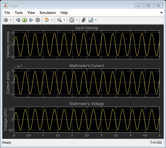
When you start the simulation, a periodic force actuates the system into a harmonic motion. The Multimeter subsystem measures the generated by the sensor current to detect this motion. Initially, you can agitate the system with a sinusoidal force to induce a simple harmonic motion. This simple test case allows assessing that the sensor is modeled accurately.

sim(myModel);
time = OscillationSensorSimlog.Sensor.Mass.v.series.time;
velocity = OscillationSensorSimlog.Sensor.Mass.v.series.values;
current = OscillationSensorSimlog.Multimeter.Current_Sensor.I.series.values;

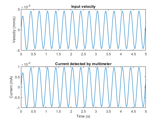
Plot the velocity and the current that the sensor generates.

figure(Name="OscillationSensorResultsFigure");
OscillationSensorPlotSignals(time,velocity,current);

The sensor is modeled accurately if the current correlates to the velocity. You can assess the extent of the correlation by calculating the correlation coefficient.

R = corrcoef(current, velocity);
format long;
disp(R(1,2));
format default;

   0.999994850155707

Compare the normalized signals

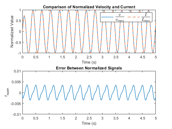
To observe how well the signals match, plot the comparison between the normalized signals. Additionally, plot the error between the normalized values. The normalized signals are strongly matching which is consistent with the high correlation coefficient. The plotted error is small at values lower than 0.005 which validates the model.

hFig = figure(Name="OscillationSensorNormalizedResultsFigure");
OscillationSensorPlotNormalizedSignals(time, velocity, current);

Test the sensor with a non-trivial harmonic force input

To assess the performance of the sensor, you can actuate the system with a force following more complex harmonic characteristics by changing the mode of the Harmonic Signal Generator block. In the second mode, the Harmonic Signal Generator block generates a complex harmonic signal by summing up two sinusoidal signals with different frequencies.

set_param(myModel+"/Harmonic Signal Generator/Mode", "Constant", "1");

sim(myModel);
time = OscillationSensorSimlog.Sensor.Mass.v.series.time;
velocity = OscillationSensorSimlog.Sensor.Mass.v.series.values;
current = OscillationSensorSimlog.Multimeter.Current_Sensor.I.series.values;

Compare the normalized signals. Similar to the simple harmonic motion, the normalized signals are strongly matching for the more complex motion. The error remains small confirming the high accuracy of the sensor.

figure(Name="OscillationSensorResultsFigure");
OscillationSensorPlotNormalizedSignals(time,velocity,current);