Analyze Battery Spatial Temperature Variation During Fast Charge
This example shows how the temperature gradient over the cell surface varies during the fast charging of a battery. Fast charging is one of the key enablers for the adoption of battery electric vehicles. Fast charging pushes a considerable amount of current inside the battery. This process produces a lot of heat. It is important to understand how temperatures spatially vary in a battery and how this affects its long term warranty. Typically, to ensure a good battery life with uniform degradation, the temperature gradient over the cell surface should not exceed around five or six degrees centigrade. This example uses Simscape™ Battery™ to model the cell electrical dynamics and the Partial Differential Equation Toolbox™ to generate the reduced order model (ROM) that describes the battery 3-D thermal model. This example uses a 50 ampere-hour battery (Valence:U27_36XP) and charges it for 10 minutes from an initial state of charge (SOC) of 15%. Then, the example analyzes the maximum gradient in the cell temperature.
Build Battery Model
To achieve optimum life and safety, the batteries on an electric vehicle are maintained between 20 and 35 °C. To avoid nonuniform degradation, you must maintain the gradient of temperature over the cell surface as low as possible. Non-uniform degradation leads to batteries fading faster than the manufacturer's specifications.

Pre-parameterize Battery
This figure shows how to parameterize the Battery (Table-Based) block with the available pre-parameterizations. For a full list of the preparameterized components in the Battery (Table-Based) block of Simscape Battery, see Predefined Parameterization.
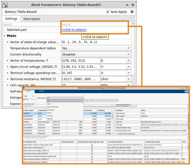
In this example, a Valence:U27_36XP battery is selected from the pre-parameterized Battery (Table-Based) block inside the Simscape Battery library. The Valence:U27_36XP battery measures 306 mm in width, 172 mm in thickness, and 225 mm in height. The positive and the negative terminals are hexagonal ports at the top of the battery casing. In this example, the enclosure thickness (3 mm) and the tab dimensions are assumed as there is enough data available.
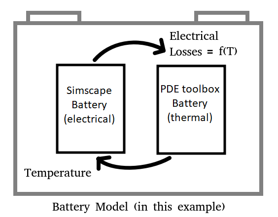
Model Battery Thermal Behavior with Partial Differential Equation Toolbox
A ROM from the Partial Differential Equation Toolbox spatially models the battery thermal behavior.
To build a 3-D model of the battery for simulation, run the sscv_setupROMmodelForSimscape live script, that uses the Partial Differential Equation Toolbox to generate a ROM from a detailed 3-D representation. The sscv_setupROMmodelForSimscape live script contains parameters to define the battery size and specify the initial conditions and the boundary conditions. All battery boundaries are adiabatic, except for the bottom surface. The bottom surface uses a function to declare thermal-resistance-based settings for the boundary.
The battery is divided into a jelly roll section, cell tabs, and the outer enclosure. The sscv_setupROMmodelForSimscape live script defines the set of thermal properties for each of these battery regions. Each region has its own separate heat generation definition. The electrical losses are computed using the Simscape Battery (Table-Based) library component block. The battery electrochemical losses from the pre-parameterized battery block are the input heat source to the jelly roll section. The tab heat source is computed based on its resistance, the current flowing through the battery, and the weld resistance defined at the junctions. The enclosure does not have any heat generation. A custom component incorporates the battery thermal model in Simscape. To generate a ROM that you can export to Simscape, run the sscv_setupROMmodelForSimscape live script. This example uses a pre-generated ROM stored inside the sscv_BatteryCellSpatialTempVariation_rom MAT file.
load('sscv_BatteryCellSpatialTempVariation_rom.mat');To update or run the ROM, at the MATLAB® Command Window, run:
edit sscv_setupROMmodelForSimscape.m
The pde_rom workspace variable comprises all data related to the ROM from the Partial Differential Equation Toolbox that defines the cell thermal model. The prop structure of the pde_rom variable defines all the physical parameters for the battery:
pde_rom.prop
ans = struct with fields:
         initialTemperature: 300
              cellTab_weldR: 7.5000e-04
            coolingArea_sqm: 0.0526
              cell_width_mm: 306
          cell_thickness_mm: 172
             cell_height_mm: 225
    cellCasing_thickness_mm: 5
          cellTab_height_mm: 8
          cellTab_radius_mm: 9
                     volume: [1×1 struct]
            cellThermalCond: [1×1 struct]
             tabThermalCond: 386
          casingThermalCond: 50
        thermalConductivity: [1×1 struct]
                    density: [1×1 struct]
                     spHeat: [1×1 struct]
            cellThermalMass: 7.0170e+03
The density, spHeat, thmCond, and volume fields of this structure contain details on the material density, specific heat, thermal conductivity, and the volume of different battery sections (jelly roll, enclosure, tabs). The cell thermal conductivities [W/m.K] in the in-plane and through-plane directions are:
pde_rom.prop.cellThermalCond
ans = struct with fields:
         inPlane: 80
    throughPlane: 2
The pde_rom.prop.thmCond.Jelly parameter sets the directionality for the battery thermal conductivity. The battery bottom cooling area is:
pde_rom.prop.coolingArea_sqm
ans =
0.0526
To visualize the battery, at the MATLAB Command Window, enter:
figure("Name","sscv_BattSpatialTempVar")
pdegplot(pde_rom.Geometry,FaceAlpha=0.3);
hold on
plot3(pde_rom.thermocouples.probe_locations(1,:),...
      pde_rom.thermocouples.probe_locations(2,:),...
      pde_rom.thermocouples.probe_locations(3,:),...
      "r*",MarkerSize=5);
hold off
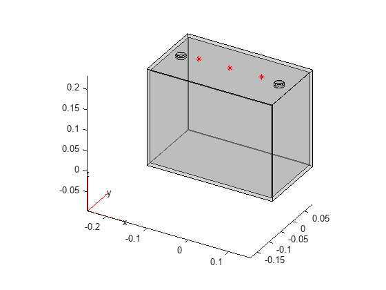
The red marks in the figure indicates that the battery has three thermocouples attached at the top. To add and define more thermocouples at any location, use the sscv_setupROMmodelForSimscape live script.
If you change the battery dimensions or thermal properties, you must regenerate the ROM. To regenerate the ROM, run the sscv_setupROMmodelForSimscape.m file with the updated battery parameters. To edit any parameter, open the sscv_setupROMmodelForSimscape.m file and apply your changes. A Simscape custom component exports the thermal model defined in pde_rom. The matrices in pde_rom are parameters for the Simscape custom component and are used to solve the energy equation in the battery.
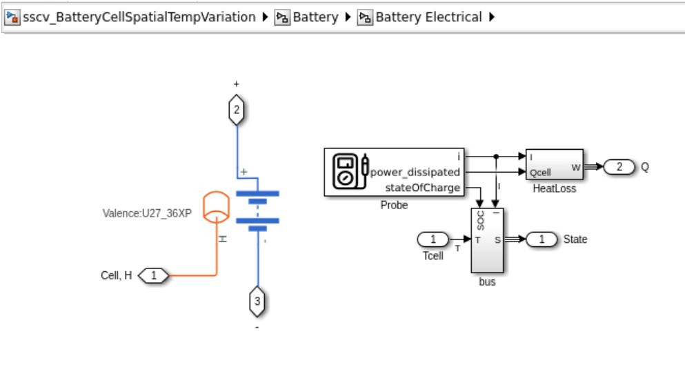
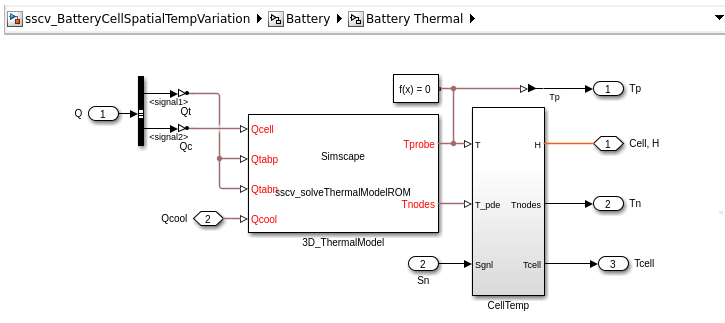
Implement Battery Electrical and Thermal Models
This figure shows how the battery electrical and thermal models are integrated in the larger circuit system in Simscape.
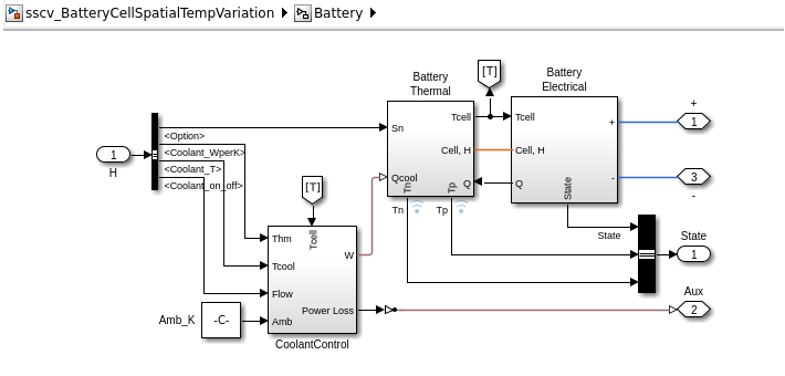
This figure shows the battery electrical and thermal modeling implementations. The Simscape custom component, 3D_ThermalModel block, contains the ROM implementation for the battery thermal modeling. The battery electrical model computes the losses for the input nodes (Qcell, Qtabp, Qtabn) of the thermal model.
The battery subsystem is ready for integration inside any circuit. After the simulation, you can reconstruct back the 3-D thermal solution from the custom component outputs. The coolant control, based on the Battery Coolant Control block from Simscape Battery, switches the flow on and off based on the cell temperature.
Simulate for Fast Charge
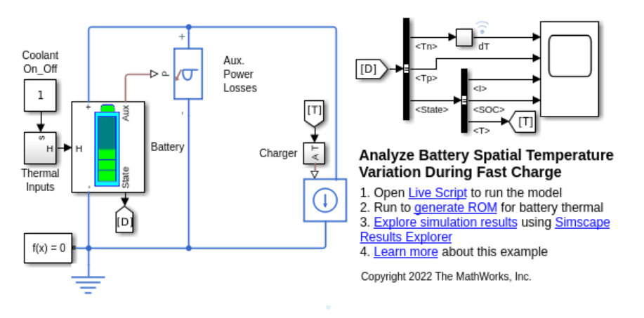
The battery connects to a Charger block that feeds in the charging current into the circuit. A time varying load is connected in parallel to the battery to account for auxiliary power requirements from the coolant pump, chiller and heater. The Option parameter in the Thermal Inputs block defines the battery electrical properties. When you set this parameter to 0, the battery temperature is equal to the average temperature of all PDE node temperatures. When you set this parameter to any value greater than one, the temperature is equal to the temperature measured from a thermocouple with the index or number you specified in the Option parameter. This is important as the thermocouples are placed on the battery surface and the core temperature might differ from the thermocouple location.
Set a simulation time of 10 minutes for a fast charge.
totalSimulationTime=600;
Set the initial conditions.
initialStateOfCharge=0.15;
coolantTemperature_K=300;
Define the heat removal rate due to cooling system design and the coolant flow.
coolantThermalR=15; % W/KSet the maximum charge rate (C rate) as a function of the cell temperature.
cellMaxCurrVec_T=[263 273 283 293 303 313]; % Temperature
cellMaxCurrVec_C=[0.5 0.75 1.0 1.5 1.9 2.2];% C rate
Set the coolant pump power loss to a constant value of 50W.
lossAuxPowSources_W=50;
Set the chiller or heater losses as a function of the coolant temperature difference with the ambient.
chillerHeaterLosses_dT=[0 20 30 40 50]; % |Tcoolant~Tambient|
chillerHeaterLosses_W=[0 5 10 15 20];   % W
Run the simulation.
sim('sscv_BattSpatialTempVar.slx')
pde_results.pde_T_values=squeeze(...
    logsout_BatteryCellSpatialTempVariation.find("Tn").Values.Data);
Simulation Results
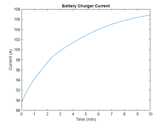
Plot the charge current with time.
plot(simlog_sscv_BattSpatialTempVar.Charger.A.series.time/60, ...
     abs(simlog_sscv_BattSpatialTempVar.Charger.A.series.values));
xlabel("Time (min)");ylabel("Current (A)");
title("Battery Charger Current");
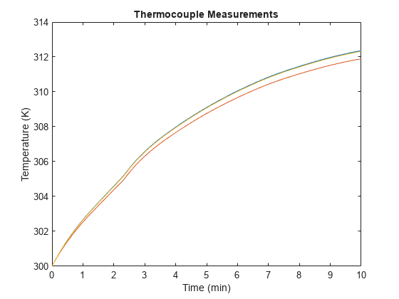
Plot the temperature measured at probe locations.
plot(logsout_BatteryCellSpatialTempVariation.find("Tp").Values.Time/60, ...
     squeeze(logsout_BatteryCellSpatialTempVariation.find("Tp").Values.Data)');
xlabel("Time (min)");ylabel("Temperature (K)");
title("Thermocouple Measurements");
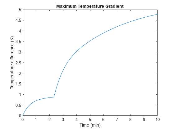
Plot the maximum temperature gradient in the battery based on all the nodal temperatures in detailed 3-D solution.
plot(logsout_BatteryCellSpatialTempVariation.find("dT").Values.Time/60, ...
     squeeze(logsout_BatteryCellSpatialTempVariation.find("dT").Values.Data)');
xlabel("Time (min)");ylabel("Temperature difference (K)");
title("Maximum Temperature Gradient");
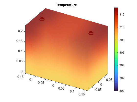
Visualize the temperature distribution in the battery cell using the Visualize PDE Results Live Editor task.
First, construct the full PDE solution using the ROM degrees-of-freedom, modal temperatures, and time data from simulation.
modalTemperature = squeeze(Tmodal.Data);
timeMinute  = logsout_BatteryCellSpatialTempVariation.find("dT").Values.Time/60;
Use ROM object in pde_rom and call the reconstructSolution method to obtain a transient thermal results object.
Rtransient = pde_rom.rom.reconstructSolution(modalTemperature,timeMinute);
On the Live Editor tab, select Task > Visualize PDE Results to insert the task. In the Select results section of the task, select Rtransient from the drop-down list.
% Data to visualize
meshData = Rtransient.Mesh;
nodalData = Rtransient.Temperature(:,601);

% Create PDE result visualization
resultViz = pdeviz(meshData,nodalData, ...
    "Title","Temperature", ...
    "ColorLimits",[300 313.1], ...
    "Transparency",0.55);
% Clear temporary variables
clearvars meshData nodalData
The maximum temperature gradient during the 10 minute charge process is equal to around 5 degrees, which is reasonable. Higher temperature gradients might lead to the redesign of the cooling system or change in the fast charge profile to limit the non-uniformity in cell degradation with time.