histogram

Plot histogram of multiparametric global sensitivity analysis results

Since R2020a

Syntax

h = histogram(mpgsaObj)

h = histogram(mpgsaObj,Name,Value)

Description

h = histogram(mpgsaObj) plots a histogram of multiparametric global sensitivity analysis (MPGSA) results and returns the figure handle h.

h = histogram(mpgsaObj,Name,Value) uses additional options specified by one or more name-value pair arguments.

Examples

Perform Multiparametric Global Sensitivity Analysis (MPGSA)

Load the target-mediated drug disposition (TMDD) model.

sbioloadproject tmdd_with_TO.sbproj

Get the active configset and set the target occupancy (TO) as the response.

cs = getconfigset(m1);
cs.RuntimeOptions.StatesToLog = 'TO';

Simulate the model and plot the TO profile.

sbioplot(sbiosimulate(m1,cs));

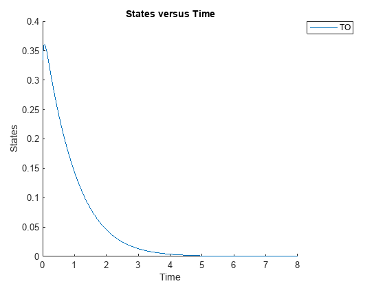
Define an exposure (area under the curve of the TO profile) threshold for the target occupancy.

classifier = 'trapz(time,TO) <= 0.1';

Perform MPGSA to find sensitive parameters with respect to the TO. Vary the parameter values between predefined bounds to generate 10,000 parameter samples.

% Suppress an information warning that is issued during simulation.
warnSettings = warning('off', 'SimBiology:sbservices:SB_DIMANALYSISNOTDONE_MATLABFCN_UCON');
rng(0,'twister'); % For reproducibility
params = {'kel','ksyn','kdeg','km'};
bounds = [0.1, 1; 
          0.1, 1;
          0.1, 1;
          0.1, 1];
mpgsaResults = sbiompgsa(m1,params,classifier,Bounds=bounds,NumberSamples=10000)

mpgsaResults = 
  MPGSA with properties:

                    Classifiers: {'trapz(time,TO) <= 0.1'}
    KolmogorovSmirnovStatistics: [4x1 table]
                       ECDFData: {4x4 cell}
              SignificanceLevel: 0.0500
                        PValues: [4x1 table]
              SupportHypothesis: [10000x1 table]
               ParameterSamples: [10000x4 table]
                    Observables: {'TO'}
                 SimulationInfo: [1x1 struct]

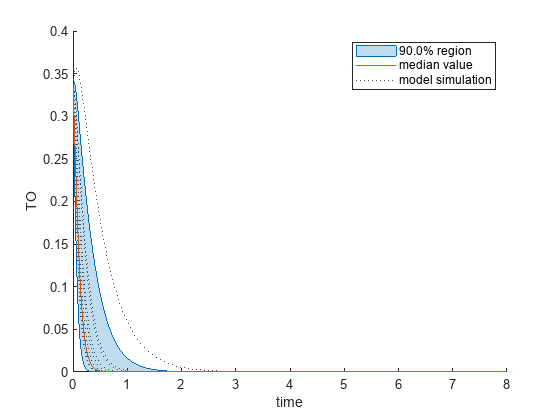
Plot the quantiles of the simulated model response.

plotData(mpgsaResults,ShowMedian=true,ShowMean=false);

Plot the empirical cumulative distribution functions (eCDFs) of the accepted and rejected samples. Except for km, none of the parameters shows a significant difference in the eCDFs for the accepted and rejected samples. The km plot shows a large Kolmogorov-Smirnov (K-S) distance between the eCDFs of the accepted and rejected samples. The K-S distance is the maximum absolute distance between two eCDFs curves.

h = plot(mpgsaResults);
% Resize the figure.
pos = h.Position(:);
h.Position(:) = [pos(1) pos(2) pos(3)*2 pos(4)*2];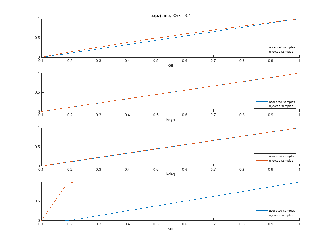

To compute the K-S distance between the two eCDFs, SimBiology uses a two-sided test based on the null hypothesis that the two distributions of accepted and rejected samples are equal. See kstest2 (Statistics and Machine Learning Toolbox) for details. If the K-S distance is large, then the two distributions are different, meaning that the classification of the samples is sensitive to variations in the input parameter. On the other hand, if the K-S distance is small, then variations in the input parameter do not affect the classification of samples. The results suggest that the classification is insensitive to the input parameter. To assess the significance of the K-S statistic rejecting the null-hypothesis, you can examine the p-values.

bar(mpgsaResults)

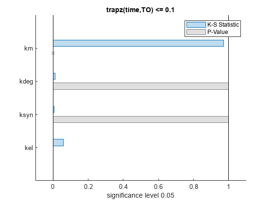
The bar plot shows two bars for each parameter: one for the K-S distance (K-S statistic) and another for the corresponding p-value. You reject the null hypothesis if the p-value is less than the significance level. A cross (x) is shown for any p-value that is almost 0. You can see the exact p-value corresponding to each parameter.

[mpgsaResults.ParameterSamples.Properties.VariableNames',mpgsaResults.PValues]

ans=4×2 table
      Var1      trapz(time,TO) <= 0.1
    ________    _____________________

    {'kel' }          0.0021877      
    {'ksyn'}                  1      
    {'kdeg'}            0.99983      
    {'km'  }                  0      

The p-values of km and kel are less than the significance level (0.05), supporting the alternative hypothesis that the accepted and rejected samples come from different distributions. In other words, the classification of the samples is sensitive to km and kel but not to other parameters (kdeg and ksyn).

You can also plot the histograms of accepted and rejected samples. The historgrams let you see trends in the accepted and rejected samples. In this example, the histogram of km shows that there are more accepted samples for larger km values, while the kel histogram shows that there are fewer rejected samples as kel increases.

h2 = histogram(mpgsaResults);
% Resize the figure.
pos = h2.Position(:);
h2.Position(:) = [pos(1) pos(2) pos(3)*2 pos(4)*2];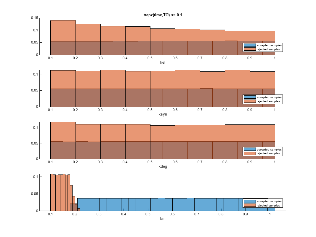

Restore the warning settings.

warning(warnSettings);

Input Arguments

mpgsaObj — Multiparametric global sensitivity analysis results

SimBiology.gsa.MPGSA object

Multiparametric global sensitivity analysis results, specified as a SimBiology.gsa.MPGSA object.

Name-Value Arguments

Specify optional pairs of arguments as Name1=Value1,...,NameN=ValueN, where Name is the argument name and Value is the corresponding value. Name-value arguments must appear after other arguments, but the order of the pairs does not matter.

Before R2021a, use commas to separate each name and value, and enclose Name in quotes.

Example: h = histogram(results,'Classifier',1) specifies to plot histograms of MPGSA results of the first classifier.

Parameters — Input model quantities to plot

character vector | string | string vector | cell array of character vectors | vector of positive integers

Input model quantities, namely parameters, species, or compartments, to plot, specified as a character vector, string, string vector, cell array of character vectors, or a vector of positive integers indexing into the columns of the mpgsaObj.ParameterSamples table.

Example: 'Parameters','k1'

Data Types: double | char | string | cell

Classifiers — Classifiers to plot

character vector | string | string vector | cell array of character vectors | vector of positive integers

Classifiers to plot, specified as a character vector, string, string vector, cell array of character vectors, or a vector of positive integers.

Specify the expressions of classifiers to plot as a character vector, string, string vector, cell array of character vectors. Alternatively, you can specify a vector of positive integers indexing into mpgsaObj.Classifiers.

Example: 'Classifiers',[1 3]

Data Types: double | char | string | cell

AcceptedSamplesColor — Color of accepted samples

three-element row vector | hexadecimal color code | color name

Color of accepted samples, specified as a three-element row vector, hexadecimal color code, color name, or a short name. By default, the function uses the first MATLAB^® default color. To view the default color order, enter get(groot,'defaultAxesColorOrder') or see the ColorOrder property.

For details on valid color names and corresponding RGB triplets and hexadecimal codes, see Specify Plot Colors.

Example: 'AcceptedSamplesColor',[0.4,0.3,0.2]

Data Types: double

RejectedSamplesColor — Color of rejected samples

three-element row vector | hexadecimal color code | color name

Color of rejected samples, specified as a three-element row vector, hexadecimal color code, color name, or a short name. By default, the function uses the second MATLAB default color. To view the default color order, enter get(groot,'defaultAxesColorOrder') or see the ColorOrder property.

For details on valid color names and corresponding RGB triplets and hexadecimal codes, see Specify Plot Colors.

Example: 'RejectedSamplesColor',[0.9,0.5,0.2]

Data Types: double

Output Arguments

h — Handle

figure handle

Handle to the figure, specified as a figure handle.

References

[1] Tiemann, Christian A., Joep Vanlier, Maaike H. Oosterveer, Albert K. Groen, Peter A. J. Hilbers, and Natal A. W. van Riel. “Parameter Trajectory Analysis to Identify Treatment Effects of Pharmacological Interventions.” Edited by Scott Markel. PLoS Computational Biology 9, no. 8 (August 1, 2013): e1003166. https://doi.org/10.1371/journal.pcbi.1003166.

Version History

Introduced in R2020a