plotResidualDistribution
Plot the distribution of the residuals
Description
plotResidualDistribution(
shows the normal probability plot and the corresponding histogram of the residuals.
Use the plot to check if the distribution of the residuals deviates from the
normality.resultsObj)
Examples
Load the sample data set.
load data10_32R.mat
gData = groupedData(data);
gData.Properties.VariableUnits = ["","hour","milligram/liter","milligram/liter"];
Create a two-compartment PK model.
pkmd                 = PKModelDesign;
pkc1                 = addCompartment(pkmd,"Central");
pkc1.DosingType      = "Infusion";
pkc1.EliminationType = "linear-clearance";
pkc1.HasResponseVariable = true;
pkc2                 = addCompartment(pkmd,"Peripheral");
model                = construct(pkmd);
configset            = getconfigset(model);
configset.CompileOptions.UnitConversion = true;
responseMap = ["Drug_Central = CentralConc","Drug_Peripheral = PeripheralConc"];
Provide model parameters to estimate.
paramsToEstimate   = ["log(Central)","log(Peripheral)","Q12","Cl_Central"];
estimatedParam     = estimatedInfo(paramsToEstimate,'InitialValue',[1 1 1 1]);
Assume every individual receives an infusion dose at time = 0, with a total infusion amount of 100 mg at a rate of 50 mg/hour.
dose             = sbiodose("dose","TargetName","Drug_Central");
dose.StartTime   = 0;
dose.Amount      = 100;
dose.Rate        = 50;
dose.AmountUnits = "milligram";
dose.TimeUnits   = "hour";
dose.RateUnits   = "milligram/hour";
Estimate model parameters. By default, the function estimates a set of parameter for each individual (unpooled fit).
fitResults = sbiofit(model,gData,responseMap,estimatedParam,dose);
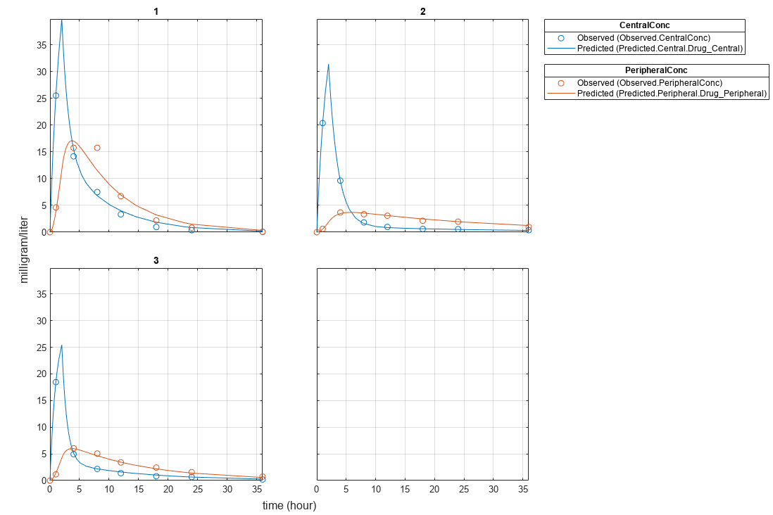
Plot the results.
plot(fitResults);
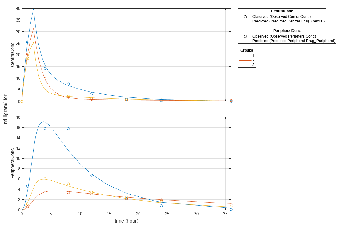
Plot all groups in one plot.
plot(fitResults,"PlotStyle","one axes");
Change some axes properties.
s = struct;
s.Properties.XGrid = "on";
s.Properties.YGrid = "on";
plot(fitResults,"PlotStyle","one axes","AxesStyle",s);

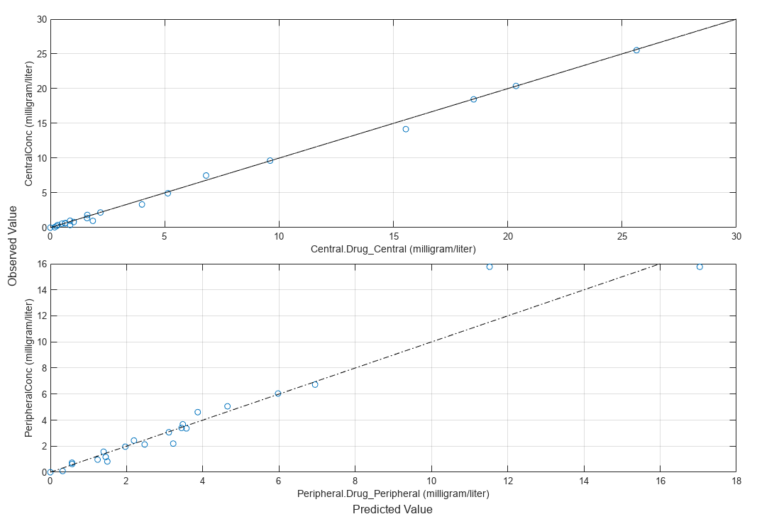
Compare the model predictions to the actual data.
plotActualVersusPredicted(fitResults);
Use boxplot to show the variation of estimated model parameters.
plotParameterStats(fitResults,"box");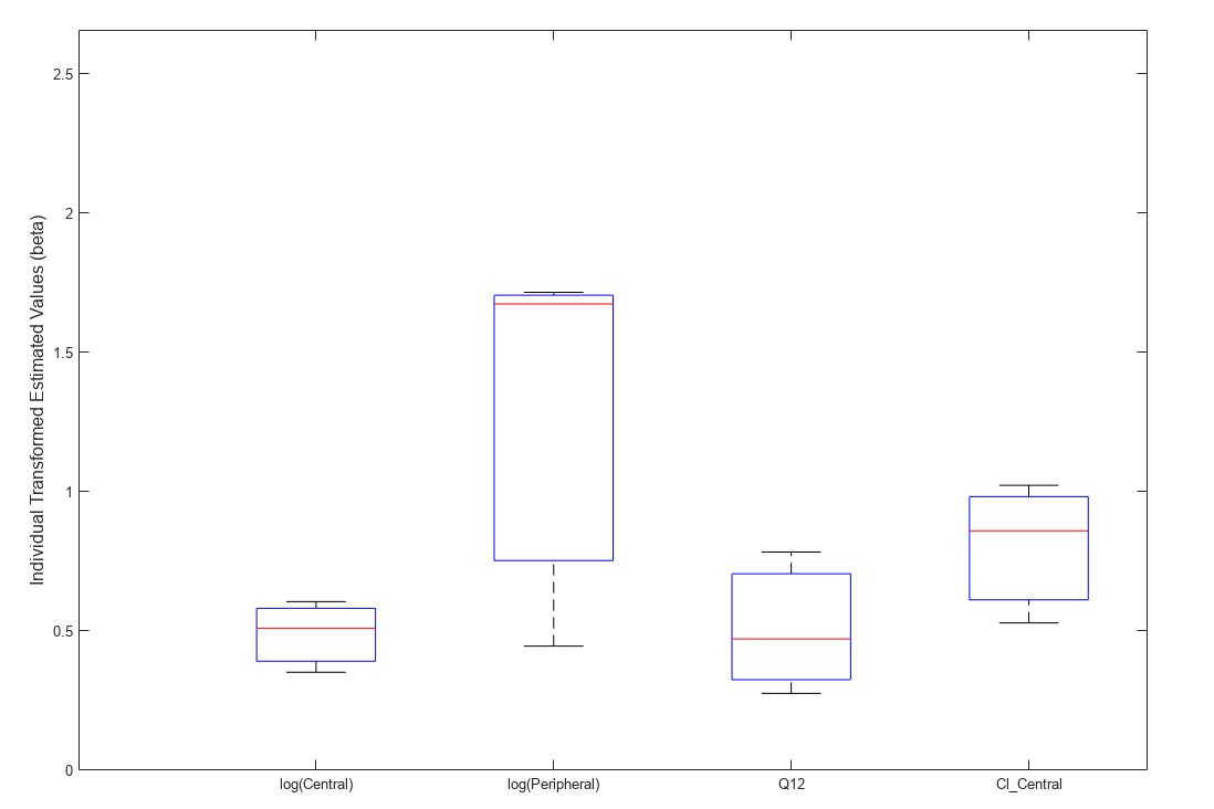
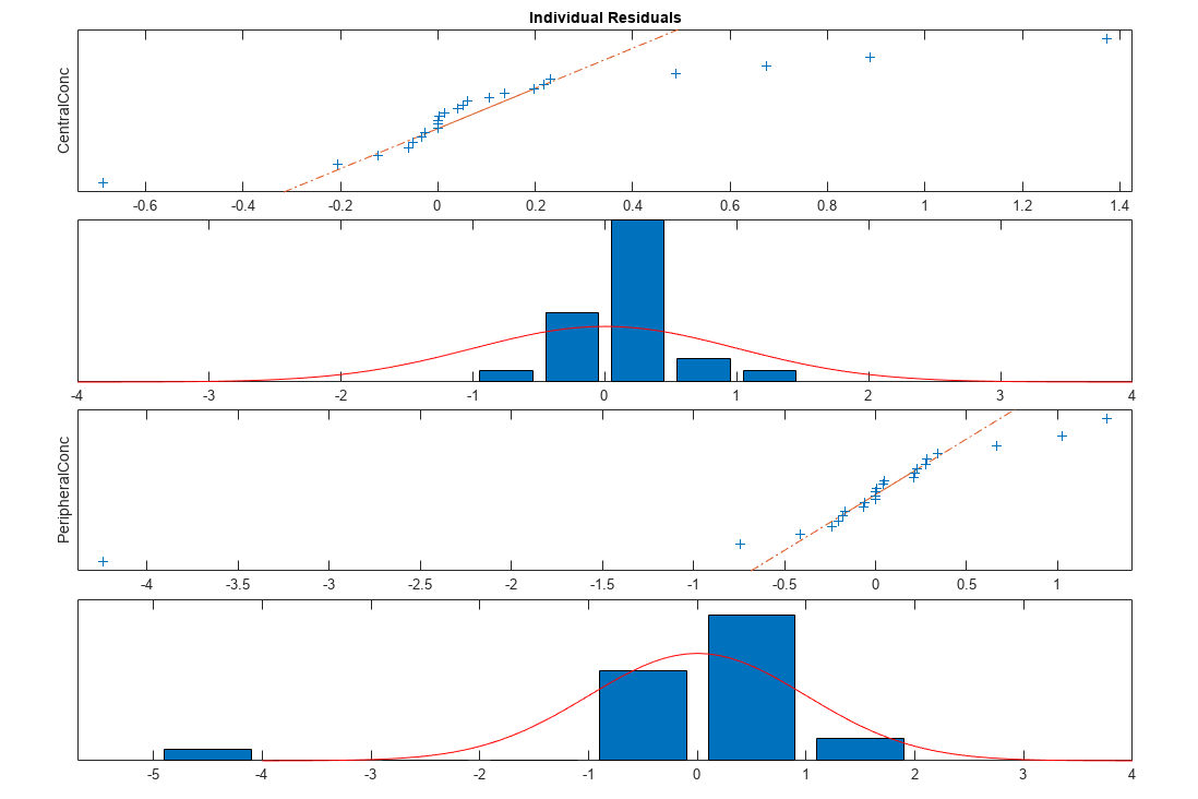
Plot the distribution of residuals. This normal probability plot shows the deviation from normality and the skewness on the right tail of the distribution of residuals. The default (constant) error model might not be the correct assumption for the data being fitted.
plotResidualDistribution(fitResults);
Plot residuals for each response using the model predictions on x-axis.
plotResiduals(fitResults,"Predictions");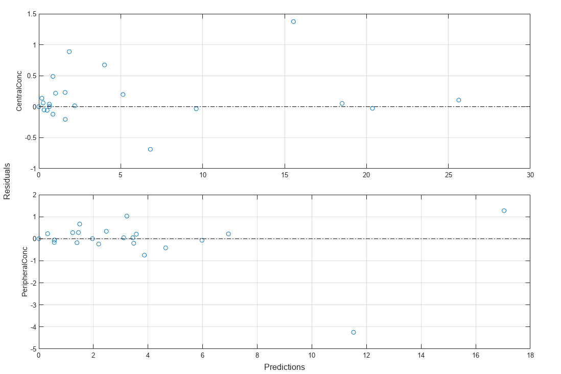
Get the summary of the fit results. stats.Name contains the name for each table from stats.Table, which contains a list of tables with estimated parameter values and fit quality statistics.
fitMetrics = summary(fitResults);
Display the table that contains parameter estimates summary statistics.
tableToShow = "Parameter Estimates Summary Statistics";
tableNames = {fitMetrics.Name};
tfShowTable = matches(tableNames,tableToShow);
disp(fitMetrics(tfShowTable).Table);
Statistic Central Peripheral Q12 Cl_Central
______________________ _______ __________ ______ __________
{'Minimum' } 1.422 0.5291 1.5619 0.2764
{'Lower Quartile' } 1.483 0.61191 2.5055 0.32521
{'Median' } 1.6657 0.86035 5.3364 0.47163
{'Upper Quartile' } 1.7906 0.98252 5.5065 0.70562
{'Maximum' } 1.8322 1.0233 5.5632 0.78361
{'Mean' } 1.64 0.80423 4.1539 0.51055
{'Standard Deviation'} 0.2063 0.25181 2.2476 0.25583
Input Arguments
Version History
Introduced in R2014a