RMS Value of Periodic Waveforms

This example shows how to find the root mean square (RMS) value of a sine wave, a square wave, and a rectangular pulse train using rms. The waveforms in this example are discrete-time versions of their continuous-time counterparts.

Create a sine wave with a frequency of $$\pi /4$$ rad/sample. The length of the signal is 16 samples, which equals two periods of the sine wave.

n = 0:15;
x = cos(pi/4*n);

Compute the RMS value of the sine wave.

rmsval = rms(x)

rmsval = 
0.7071

The RMS value is equal to $$1/\surd 2$$, as expected.

Create a periodic square wave with a period of 0.1 seconds. The square wave values oscillate between $$-2$$ and $$2$$.

t = 0:0.01:1;
x = 2*square(2*pi*10*t);

stem(t,x,'filled')
axis([0 1 -2.5 2.5])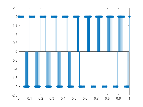

Find the RMS value.

rmsval = rms(x)

rmsval = 
2

The RMS value agrees with the theoretical value of 2.

Create a rectangular pulse train sampled at 1 kHz with the following parameters: the pulse is on, or equal to 1, for 0.025 seconds, and off, or equal to 0, for 0.075 seconds in each 0.1 second interval. This means the pulse period is 0.1 seconds and the pulse is on for 1/4 of that interval. This is referred to as the duty cycle. Use pulstran to create the rectangular pulse train.

t = 0:0.001:(10*0.1);
pulsewidth = 0.025;
pulseperiods = [0:10]*0.1;
x = pulstran(t,pulseperiods,@rectpuls,pulsewidth);

plot(t,x)
axis([0 1 -0.5 1.5])

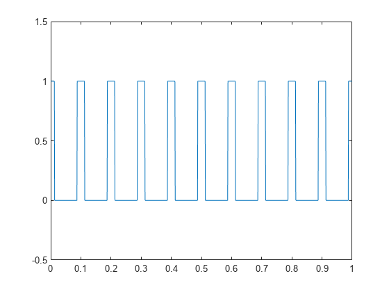
Find the RMS value and compare it to the RMS of a continuous-time rectangular pulse waveform with duty cycle 1/4 and peak amplitude 1.

rmsval = rms(x)

rmsval = 
0.5007

thrms = sqrt(1/4)

thrms = 
0.5000

The observed RMS value and the RMS value for a continuous-time rectangular pulse waveform are in good agreement.