Task-Space Motion Model
The task-space motion model characterizes the motion of a manipulator under closed-loop task-space position control, as used in the taskSpaceMotionModel object and Task Space Motion Model block.
Robot manipulators are typically position controlled devices. For task-space control, you specify a reference end-effector pose in SE(3), and the model returns the joint configuration vector and its state derivatives. You can do this by using closed-loop control on the robot joints and using the motion model to simulate the behavior of the robot under this control.
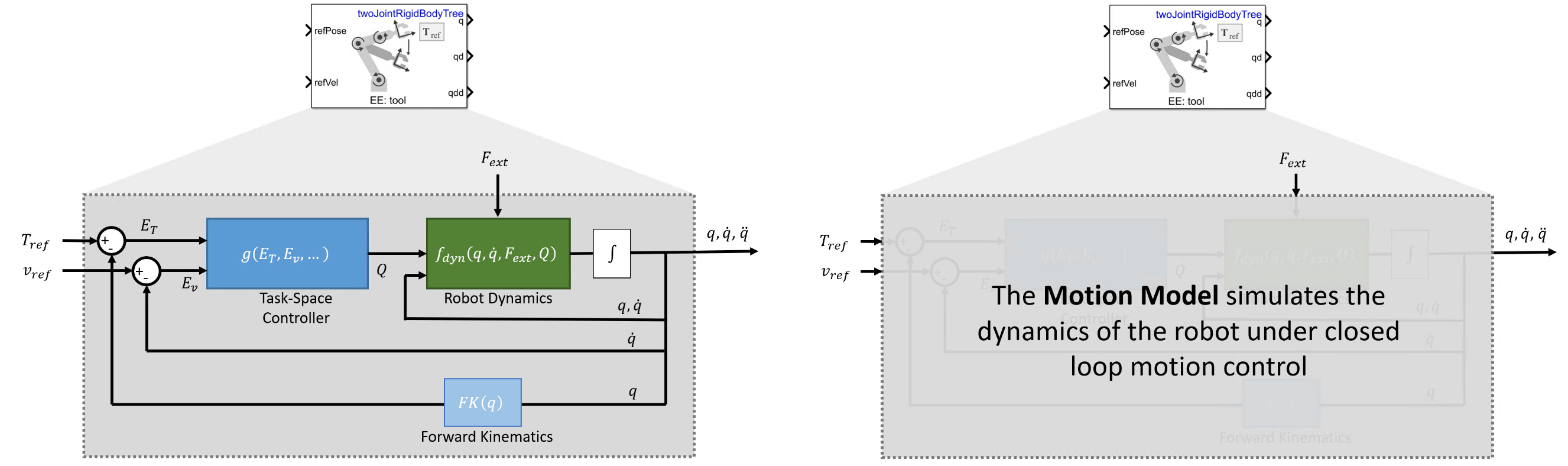
For this approach to most closely approximate the motion of the actual system, you must accurately represent the dynamics of the controller and plant. While there are many variations of task-space control, this model uses a relatively simple Jacobian-Transpose approach that is most accurate when the dynamic parameters of the robot and controller are well selected to match the desired behavior. To do this, you must understand the key parameters and motion model behavior:
Background
Joint-Space vs. Task-Space Motion Models
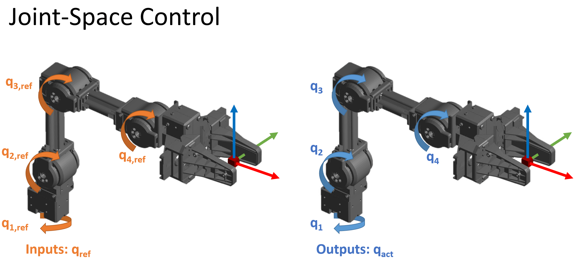
There are two categories of robot position control:
Joint-Space motion control — In this case, the position input of the robot is specified as a vector of joint angles or positions, known as the robot's joint configuration, . The controller tracks a reference configuration, , and returns the actual joint configuration . This is also known as configuration-space control.
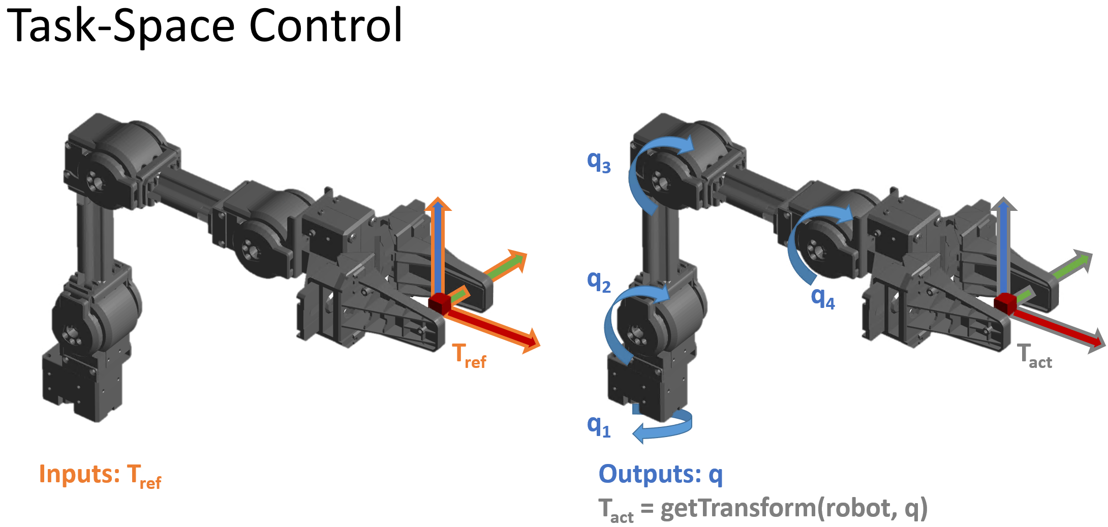
Task-Space motion control — The position is specified to a controller as an end-effector pose. Then the controller drives the robot's joint configurations to the values that move the end effector to the specified pose. This is sometimes referred to as operational-space control.
These figures shows the different types of inputs/outputs in these two motion control categories.
This topic page is specific to task-space motion control, as used in the taskSpaceMotionModel object and Task Space Motion Model block. For joint-space motion models, see the jointSpaceMotionModel object. For an example that covers the difference between task-space and joint-space control in greater detail, see Plan and Execute Task- and Joint-Space Trajectories Using Kinova Gen3 Manipulator.
Usage in MATLAB and Simulink
The task-space motion model can be represented in MATLAB® or Simulink®.
In Simulink, the Task-Space Motion Model block accepts the reference inputs and optional external force when applicable, and returns the joint configuration, velocity, and acceleration. The block handles integration, so no additional integration is required.
In MATLAB, the
taskSpaceMotionModelsystem object models the closed-loop motion. Thederivativemethod returns derivatives of the joint configuration, velocity, and acceleration at each instant in time, so you must use an ODE solver or equivalent external integration method to simulate the motion in time.
For a more specific overview, refer to the associated documentation pages.
Key Variables
The model state consists of these values:
— Robot joint configuration, as a vector of joint positions. Specified in for revolute joints and for prismatic joints.
— Vector of joint velocities in for revolute joints and for prismatic joints
— Vector of joint accelerations in for revolute joints or for prismatic joints
The end-effector pose of the robot is a 4-by-4 homogeneous matrix defined relative to the origin at the robot base. Positions are in meters. Two forms of are used for calculating errors in control:
— Reference end-effector pose, specified as a desired end-effector pose
— Actual end-effector pose achieved by the motion
The end-effector transform decomposes as:
where is the orientation as a 3-by-3 rotation matrix, and is a 3-by-1 vector of xyz-positions in meters.
The task-space velocity and acceleration consist of two 6-by-1 vectors:
,
where and are 3-by-1 vectors of angular velocities and accelerations of the frame, respectively.
Equations of Motion
Use the task-space motion model to represent robots that are subject to a control law that acts on the task-space error. For example, when the input to the control law specifies end-effector motion. While there are many ways to implement such a system, in this model, the closed-loop response is approximated in the Plan and Execute Task- and Joint-Space Trajectories Using Kinova Gen3 Manipulator object by providing a system under proportional-derivative Jacobian-Transpose style control. Regardless of how the system you are using works, this model can be used as a low-fidelity approximation of a system under closed-loop task-space control.
Proportional-Derivative Control
When the motion model uses proportional-derivative (PD) control, as determined by the MotionType property of the taskSpaceMotionModel object, the model computes forward dynamics using standard rigid body dynamics, but with subject to a PD control law that acts on the error between desired and actual end-effector pose.
Inputs — This model accepts reference pose and reference end-effector velocities
Outputs — The model returns the as the joint configuration, velocities, and accelerations as vectors
Complexity — The complexity of the model describes the overall amount of computation required. This is a medium complexity motion model. It uses complete rigid body dynamics, but the control law used in the model is relatively simple.
When it can be applied — Use the task-space motion model to represent robots that are subject to a control law that acts on the task-space error. In practice, robots are often subject to more complex task-space control laws, but the approximate behavior can still be simulated by a simplified system such as this one as long as the error dynamics behave similarly. Since this simplified control action does not contain any feedback linearization terms, it will be most accurate when tracking inputs that change gently. The model is less appropriate when compared to a more responsive controller, particularly when the reference inputs change more dynamically.
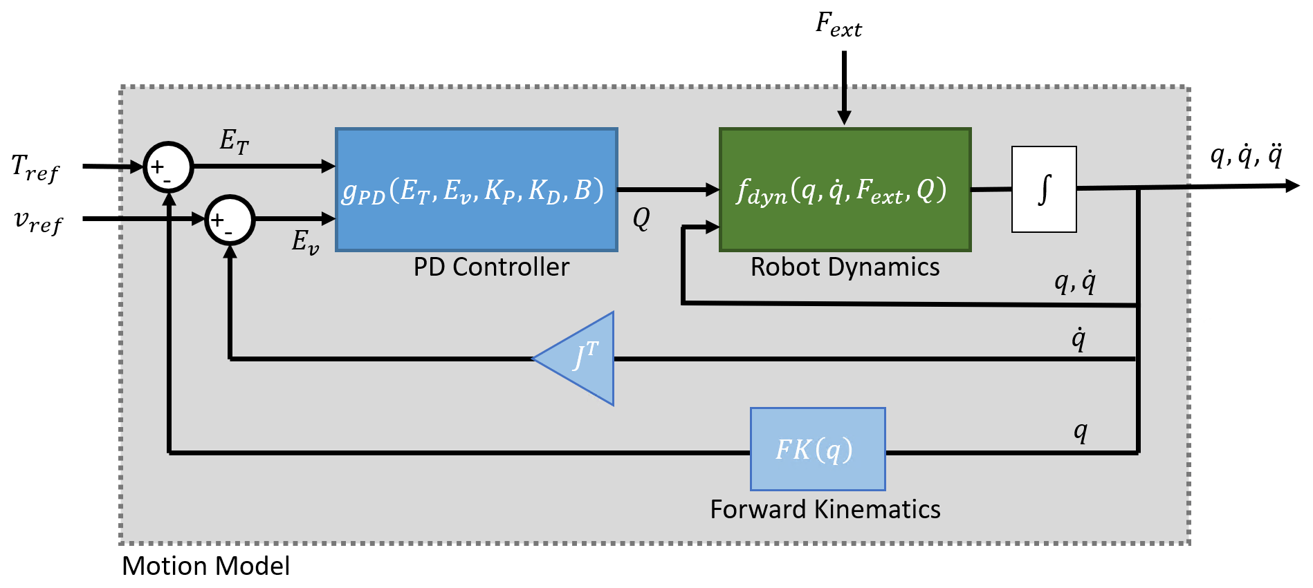
In this system, the joint positions, velocities, and accelerations are computed using standard rigid body robot dynamics. For more information, see Robot Dynamics. The generalized force input is given by the PD Control law on the task-space error, scaled to the joint-space using Jacobian-Transpose style control:
where:
— is the rotational error converted to Euler angles using
rotm2eul().— is the error in xyz-coordinates, calculated as .
— are the gravity torques and forces for all joints to maintain their positions in the specified gravity. For more information, see the
gravityTorquefunction.— is the geometric Jacobian for the given joint configuration for more information, see the
geometricJacobianfunction.
The control input relies on these user-defined parameters:
— Proportional gain, specified as a 6-by-6 matrix
— Derivative gain, specified as a 6-by-6 matrix
— Joint damping vector, specified as a two-element vector of damping constants in for revolute joints and for prismatic joints
You can specify these parameters as properties on the taskSpaceMotionModel object.
This model accepts the following inputs:
— Reference end-effector pose, specified as the desired end-effector pose
— Reference end-effector velocities, specified as a vector , with angular velocities and translational velocities