Beta
Description
Create and analyze a Beta
model object to calculate the
exposure at default (EAD) using this workflow:
Use
fitEADModel
to create aBeta
model object.Use
predict
to predict the EAD.Use
modelDiscrimination
to return AUROC and ROC data. You can plot the results usingmodelDiscriminationPlot
.Use
modelCalibration
to return the R-squared, RMSE, correlation, and sample mean error of predicted and observed EAD data. You can plot the results usingmodelCalibrationPlot
.
Creation
Description
specifies options using one or more name-value arguments in addition to the
input arguments in the previous syntax. The optional name-value arguments
set the model object properties. For example,
BetaEADModel
= fitEADModel(___,Name=Value
)BetaEADModel =
fitEADModel(EADData,ModelType,PredictorVars={'UtilizationRate','Age','Marriage'},ConversionMeasure="lcf",DrawnVar='Drawn',LimitVar='Limit',ResponseVar='EAD')
creates an BetaEADModel
object using a
Beta
model type.
Input Arguments
data
— Data for exposure at default
table
Data for exposure at default, specified as a table.
Data Types: table
ModelType
— Model type
string with value "Beta"
| character vector with value 'Beta'
Model type, specified as a string with the value of
"Beta"
or a character vector with the value of
'Beta'
.
Data Types: char
| string
Specify optional pairs of arguments as
Name1=Value1,...,NameN=ValueN
, where Name
is
the argument name and Value
is the corresponding value.
Name-value arguments must appear after other arguments, but the order of the
pairs does not matter.
Example: BetaEADModel =
fitEADModel(EADData,ModelType,PredictorVars={'UtilizationRate','Age','Marriage'},ConversionMeasure="lcf",LimitVar='Limit',ResponseVar='EAD',BoundaryTolerance=1e5)
ModelID
— User-defined model ID
"Beta"
(default) | string | character vector
User-defined model ID, specified as ModelID
and
a string or character vector. The software uses the
ModelID
text to format outputs and is
expected to be short.
Data Types: string
| char
Description
— User-defined description for model
""
(default) | string | character vector
User-defined description for model, specified as
Description
and a string or character
vector.
Data Types: string
| char
PredictorVars
— Predictor variables
all columns of data
except for
ResponseVar
(default) | string array | cell array of character vectors
Predictor variables, specified as PredictorVars
and a string array or cell array of character vectors.
PredictorVars
indicates which columns in the
data
input contain the predictor
information. By default, PredictorVars
is set to
all the columns in the data
input except for
ResponseVar
.
Data Types: string
| cell
ResponseVar
— Response variable
last column of data
(default) | string | character vector
Response variable, specified as ResponseVar
and
a string or character vector. The response variable contains the EAD
data and must be a numeric variable. By default,
ResponseVar
is set to the last column.
Data Types: string
| char
BoundaryTolerance
— Value to perturb EAD responses
1e-7
(default) | positive numeric
Value to perturb EAD response values away from 0 to 1, specified
as BoundaryTolerance
and a positive scalar
numeric.
Data Types: double
LimitVar
— Limit variable
string | character vector
Limit variable, specified as LimitVar
and a
string or character vector. LimitVar
indicates
which column in data
contains the limit amount.
The limit amount value in the data
must be a
positive numeric value. The limit depends on the loan. If the loan
is a credit card, the limit is the credit limit. If the loan is a
mortgage, the limit is the initial loan amount. In general,
LimitVar
is the maximum amount that can be
borrowed.
Note
LimitVar
is required when
ConversionMeasure
is
'lcf'
. For more information on LCF,
see Conversion Measure Options.
Data Types: string
| char
DrawnVar
— Drawn variable
string | character vector
Drawn variable, specified as DrawnVar
and a
string or character vector. DrawnVar
is the
balance on the account at the time of observation, before default,
and EAD is the balance at the time of default.
DrawnVar
indicates which column in
data
contains the drawn amount. The drawn
variable value in the data
can be a positive or
negative numeric value.
Note
When the ConversionMeasure
is
'lcf'
, DrawnVar
is
not required. In this case, DrawnVar
is
set to ""
.
Data Types: string
| char
ConversionMeasure
— Conversion measure for EAD response values
"lcf"
(default) | character vector with value 'lcf'
| string with value "lcf"
Response transform, specified as
ConversionMeasure
and a character vector or
string. Limit conversion factor (LCF) is a fraction of the limit
representing the total exposure. The EAD is then defined as the LCF
times the limit (EAD = LCF*Limit
).
For more information on LCF, see Conversion Measure Options.
Data Types: string
| char
SolverOptions
— optimoptions
object
object
Options for fitting, specified as SolverOptions
and an optimoptions
object that is created using
optimoptions
from
Optimization Toolbox™. The defaults for the optimoptions
object are:
"Display"
—"none"
"Algorithm"
—"quasi-newton"
"MaxFunctionEvaluations"
—500
✕ Number of model coefficients"MaxIterations"
— 1000
Note
When using optimoptions
with a
Beta
model, specify the
SolverName
as fminunc
.
The number of Beta
model coefficients is
determined at run time, depending on the number of predictors and
the number of categories in the categorical predictors.
Data Types: object
Properties
ModelID
— User-defined model ID
Beta
(default) | string
User-defined model ID, returned as a string.
Data Types: string
Description
— User-defined description
""
(default) | string
User-defined description, returned as a string.
Data Types: string
UnderlyingModel
— Underlying statistical model
compact linear model
This property is read-only.
Underlying statistical model, returned as a compact linear model object.
The compact version of the underlying regression model is an instance of the
risk.internal.credit.BetaModel
class.
Data Types: object
PredictorVars
— Predictor variables
all columns of data
except for the
ResponseVar
(default) | string array
Predictor variables, returned as a string array.
Data Types: string
ResponseVar
— Response variable
last column of data
(default) | string
Response variable, returned as a string.
Data Types: string
LimitVar
— Limit variable
string
Limit variable, returned as a string.
Data Types: string
DrawnVar
— Drawn variable
string
Drawn variable, returned as a string.
Data Types: string
ConversionMeasure
— Conversion measure for EAD response values
"lcf"
(default) | string with value "lcf"
Response transform, returned as a string.
Data Types: string
BoundaryTolerance
— Value to perturb LGD responses
1e-7
(default) | positive numeric
Value to perturb LGD response values away from 0 to 1, returned as a positive scalar numeric.
Data Types: double
Object Functions
predict | Predict exposure at default |
modelDiscrimination | Compute AUROC and ROC data |
modelDiscriminationPlot | Plot ROC curve |
modelCalibration | Compute R-square, RMSE, correlation, and sample mean error of predicted and observed EADs |
modelCalibrationPlot | Scatter plot of predicted and observed EADs |
Examples
Create Beta EAD Model
This example shows how to use fitEADModel
to create a Beta
model object for exposure at default (EAD).
Load EAD Data
Load the EAD data.
load EADData.mat
head(EADData)
UtilizationRate Age Marriage Limit Drawn EAD _______________ ___ ___________ __________ __________ __________ 0.24359 25 not married 44776 10907 44740 0.96946 44 not married 2.1405e+05 2.0751e+05 40678 0 40 married 1.6581e+05 0 1.6567e+05 0.53242 38 not married 1.7375e+05 92506 1593.5 0.2583 30 not married 26258 6782.5 54.175 0.17039 54 married 1.7357e+05 29575 576.69 0.18586 27 not married 19590 3641 998.49 0.85372 42 not married 2.0712e+05 1.7682e+05 1.6454e+05
rng('default'); NumObs = height(EADData); c = cvpartition(NumObs,'HoldOut',0.4); TrainingInd = training(c); TestInd = test(c);
Select Model Type
Select a model type for Beta
.
ModelType = "Beta";
Select Conversion Measure
Select a conversion measure for the EAD response values.
ConversionMeasure = "LCF";
Create Beta
EAD Model
Use fitEADModel
to create a Beta
model object using the TrainingInd
data.
BetaEADModel = fitEADModel(EADData(TrainingInd,:),ModelType,PredictorVars={'UtilizationRate','Age','Marriage'}, ... ConversionMeasure=ConversionMeasure,LimitVar="Limit",ResponseVar="EAD",BoundaryTolerance=2e-05); disp(BetaEADModel);
Beta with properties: BoundaryTolerance: 2.0000e-05 ModelID: "Beta" Description: "" UnderlyingModel: [1x1 risk.internal.credit.BetaModel] PredictorVars: ["UtilizationRate" "Age" "Marriage"] ResponseVar: "EAD" LimitVar: "Limit" DrawnVar: "" ConversionMeasure: "lcf"
Display the underlying model. The underlying model's response variable is the transformation of the EAD response data. Use the 'LimitVar'
and 'DrawnVar'
name-value arguments to modify the transformation.
disp(BetaEADModel.UnderlyingModel);
Beta regression model: logit(EAD_lcf) ~ 1_mu + UtilizationRate_mu + Age_mu + Marriage_mu log(EAD_lcf) ~ 1_phi + UtilizationRate_phi + Age_phi + Marriage_phi Estimated coefficients: Estimate SE tStat pValue __________ _________ _________ __________ (Intercept)_mu -0.68477 0.1145 -5.9807 2.5233e-09 UtilizationRate_mu 1.7029 0.077717 21.912 0 Age_mu -0.005633 0.0027489 -2.0492 0.040542 Marriage_not married_mu -0.025614 0.051927 -0.49327 0.62186 (Intercept)_phi -0.46429 0.095343 -4.8697 1.1838e-06 UtilizationRate_phi 0.41621 0.06701 6.2112 6.0945e-10 Age_phi -0.001282 0.0023262 -0.55113 0.58159 Marriage_not married_phi 0.00014849 0.042884 0.0034625 0.99724 Number of observations: 2627 Log-likelihood: -2931.19
Predict EAD
EAD prediction operates on the underlying compact statistical model and then transforms the predicted values back to the EAD scale. You can specify the predict
function with different options for the 'ModelLevel'
name-vale argument.
predictedEAD = predict(BetaEADModel,EADData(TestInd,:))
predictedEAD = 1751×1
105 ×
0.1758
0.1029
0.1528
0.0832
0.3261
0.5148
0.0648
0.0531
0.0712
0.3215
⋮
Validate EAD Model
For model validation, use modelDiscrimination
, modelDiscriminationPlot
, modelCalibration
, and modelCalibrationPlot
.
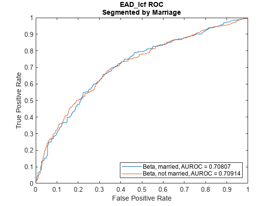
Use modelDiscrimination
and then modelDiscriminationPlot
to plot the ROC curve.
ModelLevel = "ConversionMeasure"; [DiscMeasure1,DiscData1] = modelDiscrimination(BetaEADModel,EADData(TestInd,:),ModelLevel=ModelLevel); modelDiscriminationPlot(BetaEADModel,EADData(TestInd, :),ModelLevel=ModelLevel,SegmentBy="Marriage");
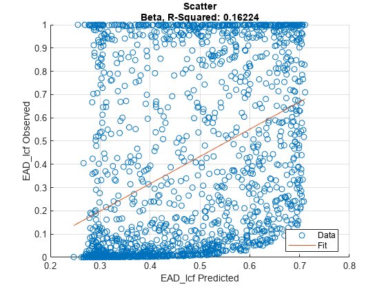
Use modelCalibration
and then modelCalibrationPlot
to show a scatter plot of the predictions.
YData = "Observed";
[CalMeasure1,CalData1] = modelCalibration(BetaEADModel,EADData(TestInd,:),ModelLevel=ModelLevel);
modelCalibrationPlot(BetaEADModel,EADData(TestInd,:),ModelLevel=ModelLevel,YData=YData);
Plot a histogram of observed EAD with respect to the predicted EAD.
figure; histogram(CalData1.Observed); hold on; histogram(CalData1.(('Predicted_' + ModelType))); legend('Observed','Predicted');
More About
Beta
Regression Models
Beta regression models model continuous variables that assume values in the open standard unit interval (0, 1).
The beta regression model is based on the assumption that the dependent variable is beta-distributed and that its mean is related to a set of regressors through a linear predictor with unknown coefficients and a link function. The beta regression model also includes a precision parameter that may be constant or depend on a potentially different set of regressors through a link function as well.
If the variable takes on values in (a, b) with a < b, you can model (y - a) / (b - a). Also, if y also assumes the extremes 0 and 1, a useful transformation in practice is y (n - 1) + 0.5) / n, where n is the sample size.
The beta regression model is based on an alternative parameterization of the beta density in terms of the mean and a precision parameter: μ = a / (a + b) and φ = a + b, 0 < μ < 1, φ > 0.
The beta regression model is defined as
where β = (β0,β1,…,βk)T, ᵞ = (ᵞ0,ᵞ1,…,ᵞk)T are the regression coefficients, η1i, η2i are the linear predictors, and xi, zi are the independent variables. g1 and g2 are the link functions where g1 is logit and g2 is log.
Parameter estimation is performed by maximum likelihood (ML).
References
[1] Baesens, Bart, Daniel Roesch, and Harald Scheule. Credit Risk Analytics: Measurement Techniques, Applications, and Examples in SAS. Wiley, 2016.
[2] Bellini, Tiziano. IFRS 9 and CECL Credit Risk Modelling and Validation: A Practical Guide with Examples Worked in R and SAS. San Diego, CA: Elsevier, 2019.
[3] Brown, Iain. Developing Credit Risk Models Using SAS Enterprise Miner and SAS/STAT: Theory and Applications. SAS Institute, 2014.
[4] Roesch, Daniel and Harald Scheule. Deep Credit Risk. Independently published, 2020.
Version History
Introduced in R2022bR2023a: modelAccuracy
object function is renamed to modelCalibration
function
The modelAccuracy
object function is renamed to
modelCalibration
function. The use of
modelAccuracy
is discouraged, use modelCalibration
instead.
R2023a: modelAccuracyPlot
object function is renamed to modelCalibrationPlot
function
The modelAccuracyPlot
object function is renamed to
modelCalibrationPlot
function. The use of
modelAccuracyPlot
is discouraged, use modelCalibrationPlot
instead.
See Also
Functions
MATLAB-Befehl
Sie haben auf einen Link geklickt, der diesem MATLAB-Befehl entspricht:
Führen Sie den Befehl durch Eingabe in das MATLAB-Befehlsfenster aus. Webbrowser unterstützen keine MATLAB-Befehle.
Select a Web Site
Choose a web site to get translated content where available and see local events and offers. Based on your location, we recommend that you select: .
You can also select a web site from the following list:
How to Get Best Site Performance
Select the China site (in Chinese or English) for best site performance. Other MathWorks country sites are not optimized for visits from your location.
Americas
- América Latina (Español)
- Canada (English)
- United States (English)
Europe
- Belgium (English)
- Denmark (English)
- Deutschland (Deutsch)
- España (Español)
- Finland (English)
- France (Français)
- Ireland (English)
- Italia (Italiano)
- Luxembourg (English)
- Netherlands (English)
- Norway (English)
- Österreich (Deutsch)
- Portugal (English)
- Sweden (English)
- Switzerland
- United Kingdom (English)