rffilter
Create Butterworth, Chebyshev, and inverse Chebyshev RF filter
Description
Use the rffilter object to create a Butterworth, Chebyshev
or an Inverse Chebyshev RF filter. The RF filter is a two-port circuit object, and you
can include this object as an element of a circuit. For more design information see,
Parameters to Define Filter and Design Tips.
You can also convert the rffilter object to a LC ladder filter by
using the lcladder
object. For example, LCLad = lcladdder(rffiltobj) where
rffiltobj is an rffilter object.
Creation
Properties
Filter type, specified as "Butterworth",
"Chebyshev", or
"InverseChebyshev".
Example: FilterType="Chebyshev"
Example: rfobj.FilterType = "Chebyshev"
Data Types: char | string
Filter response type, specified as "Lowpass",
"Highpass", "Bandpass", or
"Bandstop". For more information, see Frequency Responses.
Example: ResponseType="Highpass"
Example: rfobj.ResponseType = "Highpass"
Data Types: char | string
Filter implementation, specified as "LC Tee",
"LC Pi", or "Transfer
function".
Example: Implementation="Transfer
function"
Example: rfobj.Implementation = "Transfer function"
Dependencies
For Inverse Chebyshev type filter, you can only use
"Transfer function" implementation.
Data Types: char | string
Filter order, specified as a real finite non-negative integer. In a lowpass or highpass filter, the order specifies the number of lumped storage elements. In a bandpass or bandstop filter, the number of lumped storage elements is twice the value of the order.
Note
FilterOrder has the highest precedence among
all the name-value pairs in the filter design. Using this property
sets the UseFilterOrder read-only property to
true.
Example: FilterOrder=4
Example: rfobj.FilterOrder = 4
Data Types: double
Passband frequency, specified as:
A scalar in hertz for lowpass and highpass filters.
A two-element vector in hertz for bandpass or bandstop filters.
By default, the values are 1e9 for lowpass
filter, 2e9 for highpass filter, and [2e9
3e9] for bandpass and [[1e9 4e9] for
bandstop filters.
Example: PassbandFrequency=[3e6 5e6]
Example: rfobj.PassbandFrequency = [3e6
5e6]
Data Types: double
Stopband frequency, specified as:
A scalar in hertz for lowpass and highpass filters.
A two-element vector in hertz for bandpass or bandstop filters.
By default, the values are 2e9 for lowpass
filter, 1e9 for highpass filter, [1.5e9
3.5e9] for bandpass filters, and [2.1e9
2.9e9] bandstop filters.
Example: rffilter(ResponseType="lowpass",StopbandFrequency=[3e6
5e6])
Example: rfobj.StopbandFrequency = [3e6
5e6]
Data Types: double
Passband attenuation, specified as a scalar in dB. For bandpass filters, this value is applied equally to both edges of the passband.
Example: PassbandAttenuation=5
Example: rfobj.PassbandAttenuation = 5
Data Types: double
Stopband attenuation, specified as a scalar in dB. For bandstop filters, this value is applied equally to both edges of the stopband.
Example: StopbandAttenuation=30
Example: rfobj.StopbandAttenuation = 30
Data Types: double
Source impedance, specified as a positive real part finite scalar in ohms.
Example: Zin=70
Example: rfobj.Zin = 70
Data Types: double
Load impedance, specified as a positive real part finite scalar in ohms.
Example: Zout=70
Example: rfobj.Zout = 70
Data Types: double
Name of RF filter object, specified as a character vector. Two elements in the same circuit cannot have the same name. All names must be valid MATLAB® variable names.
Example: Name="filter1"
Example: rfobj.Name = "filter1"
Data Types: char | string
Number of ports, specified as a 2. This property is
read-only.
Data Types: double
Names of the terminals, specified as a {'p1+','p2+','p1-','p2-'}. This property is read-only.
Data Types: char
Filter design data, specified as a structure. This property is read-only. For more information, see Design Data for LC Tee and LC Pi Topologies and Design Data for Transfer Function Implementation.
Data Types: struct
Use of filter order for filter design, specified as a
true or false. This property is a
read-only.
Data Types: logical
Object Functions
groupdelay | Group delay of S-parameter, RF filter, or RF Toolbox circuit object |
sparameters | Calculate S-parameters for RF data, network, circuit, and matching network objects |
set | Set rffilter object property values |
zpk | Converts rffilter to zero-pole-gain representation |
tf | Converts rffilter to transfer function |
lcladder | Create LC ladder network |
rfplot | Plot S-parameter data |
clone | Create copy of existing circuit element or circuit object |
circuit | Circuit object |
Examples
Create and view the properties of a default RF filter object.
rfobj = rffilter
rfobj =
  rffilter: Filter element

             FilterType: 'Butterworth'
           ResponseType: 'Lowpass'
         Implementation: 'LC Tee'
            FilterOrder: 3
      PassbandFrequency: 1.0000e+09
    PassbandAttenuation: 3.0103
                    Zin: 50
                   Zout: 50
             DesignData: [1×1 struct]
         UseFilterOrder: 1
                   Name: 'Filter'
rfobj.DesignData
ans = struct with fields:
            FilterOrder: 3
              Inductors: [7.9577e-09 7.9577e-09]
             Capacitors: 6.3662e-12
               Topology: 'lclowpasstee'
      PassbandFrequency: 1.0000e+09
    PassbandAttenuation: 3.0103
Create a Butterworth passband filter object named BFCG_162W with passband frequencies between 950 and 2200 MHz, stopband frequencies between 770 and 3000 MHz, passband attenuation of 3.0 dB, and stopband attenuation of 40 dB using 'LC Tee' implementation type. Calculate the S-parameters of the filter at 2.1 GHz.
robj = rffilter(ResponseType="Bandpass",Implementation="LC Tee",PassbandFrequency=[950e6 2200e6],                        ...
    StopbandFrequency=[770e6 3000e6],PassbandAttenuation=3,StopbandAttenuation=40);
robj.Name = 'BFCG_162W'
robj =
  rffilter: Filter element

             FilterType: 'Butterworth'
           ResponseType: 'Bandpass'
         Implementation: 'LC Tee'
      PassbandFrequency: [950000000 2.2000e+09]
    PassbandAttenuation: 3
      StopbandFrequency: [770000000 3.0000e+09]
    StopbandAttenuation: 40
                    Zin: 50
                   Zout: 50
             DesignData: [1×1 struct]
         UseFilterOrder: 0
                   Name: 'BFCG_162W'
Calculate the S-parameters at 2.1 GHz.
s = sparameters(robj,2.1e9)
s =
  sparameters with properties:

      Impedance: 50
       NumPorts: 2
     Parameters: [2×2 double]
    Frequencies: 2.1000e+09
Build a lcladder object from the rffilter object. This lcladder object can be used in a circuit directly and could also be used for parametric analysis across inductor and capacitance values.
l = lcladder(robj)
l =
  lcladder: LC Ladder element

        Topology: 'bandpasstee'
     Inductances: [1.8116e-09 5.7297e-09 8.3361e-09 2.8294e-09 1.2214e-08 2.3802e-09 1.2214e-08 2.8294e-09 8.3361e-09 5.7297e-09 1.8116e-09]
    Capacitances: [6.6900e-12 2.1152e-12 1.4539e-12 4.2835e-12 9.9228e-13 5.0919e-12 9.9228e-13 4.2835e-12 1.4539e-12 2.1152e-12 6.6900e-12]
            Name: 'lcfilt'
Alternatively, to access the inductors and capacitors directly from the filter object use:
L = robj.DesignData.Inductors;
C = robj.DesignData.Capacitors;
Create a Chebyshev lowpass filter with a passband frequency of 2 GHz.
robj = rffilter(FilterType="Chebyshev",PassbandFrequency=2e9);Set the filter order to 5 and the implementation to LC Pi.
set(robj,FilterOrder=5,Implementation="LC Pi");Calculate the group delay of the filter at 1.9 GHz.
groupdelay(robj,1.9e9)
ans =
1.4403e-09
This example shows how to design a low-pass Butterworth filter with passband frequency of 3 kHz, stopband frequency 7 kHz, passband attenuation of 2 dB, and stopband attenuation 60 dB. Display the filter order of such a designed filter and determine the passband frequency at 3.0103 dB. See [2] in rffilter object page.
Filter Parameters
Fp = 3e3;          % Passband frequency, Hz
Ap = 2;            % Passband attenuation, dB
Fs = 7e3;          % Stopband frequency, Hz
As = 60;           % Stopband attenuation, dB
Design Filter
r = rffilter(FilterType="Butterworth",ResponseType="Lowpass",Implementation="Transfer function",PassbandFrequency=Fp,     ...
    PassbandAttenuation=Ap,StopbandFrequency=Fs,StopbandAttenuation=As);
Filter Order of Designed Filter
N = r.DesignData.FilterOrder;
sprintf('Calculated filter order is %d',N)
ans = 'Calculated filter order is 9'
Frequency at 3.0103 dB
F_3dB = r.DesignData.PassbandFrequency/1e3;
sprintf('Frequency at 3.0103 dB is %d kHz',F_3dB)
ans = 'Frequency at 3.0103 dB is 3.090733e+00 kHz'
Visualize Magnitude Response
frequencies = linspace(0,2*Fs,1001);
rfplot(r, frequencies)

Note: To use rfplot and plot on the same figure use setrfplot. Type 'help setrfplot' in command window for information.
Reference
Larry D. Paarmann, Design and Analysis of Analog Filters: A Signal Processing Perspective, Kluwer Academic Publishers
Design a low-pass Chebyshev filter with 0.1 dB bandpass ripple, cut-off frequency of 1 rad/sec, and 50 dB attenuation at 1.1 rad/sec. Display the filter order of this designed filter [1].
Define Parameters
Fp = 1/(2*pi);          % Passband frequency, Hz
Rp = 0.1;               % Ripple in Passband, dB
Fs = 1.1/(2*pi);        % Stopband frequency, Hz
As = 50;                % Stopband attenuation, dB
Design Filter
r = rffilter(FilterType="Chebyshev",ResponseType="Lowpass",Implementation="Transfer function",PassbandFrequency=Fp,     ...
    PassbandAttenuation=Rp,StopbandFrequency=Fs,StopbandAttenuation=As)
r =
  rffilter: Filter element

             FilterType: 'Chebyshev'
           ResponseType: 'Lowpass'
         Implementation: 'Transfer function'
      PassbandFrequency: 0.1592
    PassbandAttenuation: 0.1000
      StopbandFrequency: 0.1751
    StopbandAttenuation: 50
                    Zin: 50
                   Zout: 50
             DesignData: [1×1 struct]
         UseFilterOrder: 0
                   Name: 'Filter'
Filter Order of Designed Filter
N = r.DesignData.FilterOrder;
sprintf('Calculated filter order is %d',N)
ans = 'Calculated filter order is 19'
Reference
G.Ellis, Michael,Sr.Electronic Filter Analysis and Synthesis, Artech House, 1994.
Design even order Chebyshev filter and plot the filter's frequency response.
Frequency Response of Even Order Chebyshev Filter Using Transfer Function Implementation
Design even order Chebyshev filter with specified parameters.
Fp = 3e9;          % Passband frequency, GHz
Rp = 10;           % Passband attenuation, dB
Fs = 7e9;          % Stopband frequency, GHz
As = 50;           % Stopband attenuation, dB
rffiltobj = rffilter(FilterType="Chebyshev",ResponseType="Lowpass",Implementation="Transfer function",PassbandFrequency=Fp, ...
    PassbandAttenuation=Rp,StopbandAttenuation=As,StopbandFrequency=Fs);
Plot the frequency response of even order Chebyshev filter using rfplot function.
rfplot(rffiltobj,linspace(0,7.5e9,1001))
Visualize the stopband and passband attenuation using plot function.
hold on;
plot([0 7.5], repmat([-rffiltobj.PassbandAttenuation -rffiltobj.StopbandAttenuation],2,1),'--')

Use DesignData parameter to verify the order of your filter.
N = rffiltobj.DesignData.FilterOrder;
sprintf("Calculated filter order is %d",N)
ans = "Calculated filter order is 4"
More About
For LC Tee or Pi topologies, DesignData
returns inductor and capacitor values. In addition, DesignData
includes other design parameters relevant to response type.
Lowpass/Highpass Response: Filter order, Passband Frequency, Passband Attenuation
Bandpass Response: Filter order, Passband Frequency, Passband Attenuation, Auxiliary (Wx).
Bandstop Response: Filter order, Stopband Frequency, Passband Attenuation, Auxiliary (Wx).
For bandstop response, Wx is an adjustment for the first frequency at which the lowpass prototype meets the prescribed bandstop loss. For bandpass response, Wx is an adjustment of specification of passband attenuation not equal to 3 dB. For more information, see [1].
For transfer function implementation,
DesignData returns factored polynomial coefficients for
S-parameters. These factors group the complex conjugate terms to preserve precision.
All S-parameters have a common denominator present in
Denominator. The numerator terms for S11,
S22, and S21
(S21 = S12) can be evaluated using
the factored polynomial present in numerators Numerator11,
Numerator22, and Numerator21,
respectively.
For example, consider a default lowpass filter at 1 GHz. You can find the S21 data at 1 GHz for the filter as follows:
r = rffilter(Implementation="Transfer function");
f = 1e9;
num21 = [polyval(r.DesignData.Numerator21(1,:),1i*2*pi*f) ...
        polyval(r.DesignData.Numerator21(2,:),1i*2*pi*f)];
den = [polyval(r.DesignData.Denominator(1,:),1i*2*pi*f) ...
      polyval(r.DesignData.Denominator(2,:),1i*2*pi*f)];
s21_1GHz = prod(num21./den,2)
s21_1GHz =

  -0.5000 - 0.5000i
sparameters function to calculate the
example:S = sparameters(r,1e9); S.Parameters(2,1)
ans =

  -0.5000 - 0.5000i
In addition, DesignData includes other design parameters
relevant to response type for:
Lowpass/Highpass Response: Filter order, Passband Frequency, Auxiliary (Numerator21 Polynomial)
Note
Passband frequency is at 3 dB for Butterworth filter.
Bandpass Response: Filter order, Passband Frequency, Auxiliary (Wx, Numerator21 Polynomial)
Bandstop Response: Filter order, Stopband Frequency, Auxiliary (Wx, Numerator21 Polynomial)
For bandstop response, Wx is an adjustment for the first frequency at which the lowpass prototype meets the prescribed bandstop loss. For bandpass response, Wx is an adjustment of specification of passband attenuation not equal to 3 dB.
Some additional design tips:

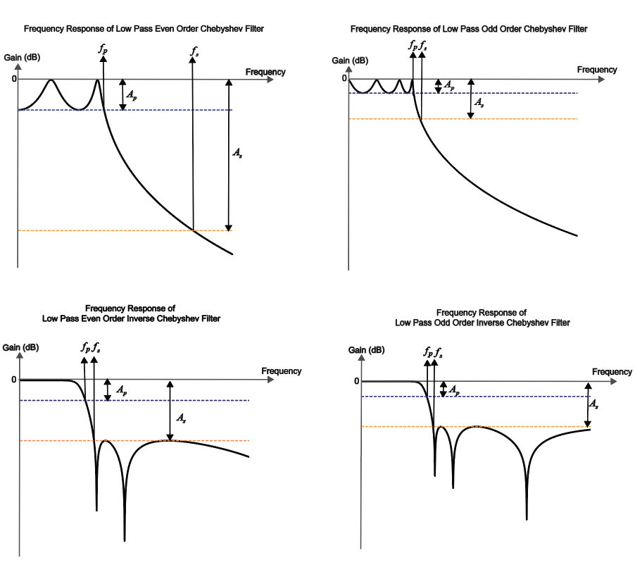
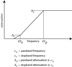
| Filter Type | Frequency Response |
|---|---|
| Lowpass |
|
| Highpass |
|
| Bandpass |
|
| Bandstop |
|

This table shows all the parameters required to design each filter correctly:

References
[1] G.Ellis, Michael,Sr.Electronic Filter Analysis and Synthesis,Artech House, 1994
[2] Larry D. Paarmann, Design and Analysis of Analog Filters, A Signal Processing Perspective with MATLAB Examples, Kluwer Academic Publishers, 2001.
Version History
Introduced in R2018b
MATLAB Command
You clicked a link that corresponds to this MATLAB command:
Run the command by entering it in the MATLAB Command Window. Web browsers do not support MATLAB commands.
Website auswählen
Wählen Sie eine Website aus, um übersetzte Inhalte (sofern verfügbar) sowie lokale Veranstaltungen und Angebote anzuzeigen. Auf der Grundlage Ihres Standorts empfehlen wir Ihnen die folgende Auswahl: .
Sie können auch eine Website aus der folgenden Liste auswählen:
So erhalten Sie die bestmögliche Leistung auf der Website
Wählen Sie für die bestmögliche Website-Leistung die Website für China (auf Chinesisch oder Englisch). Andere landesspezifische Websites von MathWorks sind für Besuche von Ihrem Standort aus nicht optimiert.
Amerika
- América Latina (Español)
- Canada (English)
- United States (English)
Europa
- Belgium (English)
- Denmark (English)
- Deutschland (Deutsch)
- España (Español)
- Finland (English)
- France (Français)
- Ireland (English)
- Italia (Italiano)
- Luxembourg (English)
- Netherlands (English)
- Norway (English)
- Österreich (Deutsch)
- Portugal (English)
- Sweden (English)
- Switzerland
- United Kingdom (English)


