Train Multiple Agents to Perform Collaborative Task
This example shows how to set up a multiagent decentralized or centralized training with a Simulink® environment. In the example, you train two agents to collaboratively perform the task of moving an object.
Fix Random Number Stream for Reproducibility
The example code might involve computation of random numbers at several stages. Fixing the random number stream at the beginning of some sections in the example code preserves the random number sequence in the section every time you run it, which increases the likelihood of reproducing the results. For more information, see Results Reproducibility.
Fix the random number stream with seed 0 and random number algorithm Mersenne twister. For more information on controlling the seed used for random number generation, see rng.
previousRngState = rng(0,"twister");The output previousRngState is a structure that contains information about the previous state of the stream. You will restore the state at the end of the example.
Environment Description
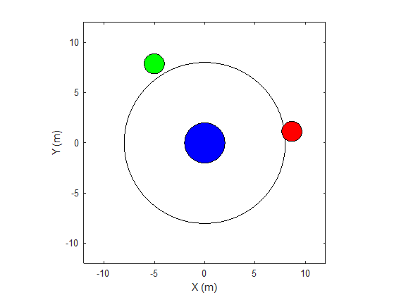
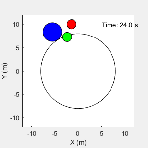
The environment in this example is a frictionless two dimensional surface containing elements represented by circles. A target object C is represented by the blue circle with a radius of 2 m, and robots A (red) and B (green) are represented by smaller circles with radii of 1 m each. The robots attempt to move object C outside a circular ring of a radius 8 m by applying forces through collision. All elements within the environment have mass and obey Newton's laws of motion. In addition, contact forces between the elements and the environment boundaries are modeled as spring and mass damper systems. The elements can move on the surface through the application of externally applied forces in the X and Y directions. The elements do not move in the third dimension and the total energy of the system is conserved.
Create the variables required for this example using the rlCollaborativeTaskParams Script.
rlCollaborativeTaskParams
Open the Simulink model.
mdl = "rlCollaborativeTask";
open_system(mdl)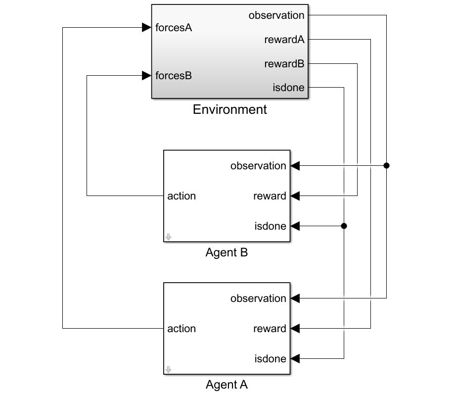
For this environment:
The 2-dimensional space is bounded from –12 m to 12 m in both the X and Y directions.
The contact spring stiffness and damping values are 100 N/m and 0.1 N/m/s, respectively.
The agents share the same observations for positions, velocities of A, B, and C and the action values from the last time step.
The simulation terminates when object C moves outside the circular ring.
At each time step, the agents receive the following reward:
Here:
and are the rewards received by agents A and B, respectively.
is a team reward that is received by both agents as object C moves closer toward the boundary of the ring.
and are local penalties received by agents A and B based on their distances from object C and the magnitude of the action from the last time step.
is the distance of object C from the center of the ring.
and are the distances between agent A and object C and agent B and object C, respectively.
The agents apply external forces on the robots that result in motion. and are the action values of the two agents A and B from the last time step. The range of action values is between -1 and 1.
Create Environment Object
To create a multiagent environment, specify the block paths of the agents using a string array. Also, specify the observation and action specification objects using cell arrays. The order of the specification objects in the cell array must match the order specified in the block path array. When agents are available in the MATLAB® workspace at the time of environment creation, the observation and action specification arrays are optional. For more information on creating multiagent environments, see rlSimulinkEnv.
Create the I/O specifications for the environment. In this example, the agents are homogeneous and have the same I/O specifications.
% Number of observations
numObs = 16;

% Number of actions
numAct = 2;

% Maximum value of externally applied force (N)
maxF = 1.0;

% I/O specifications for each agent
oinfo = rlNumericSpec([numObs,1]);
ainfo = rlNumericSpec([numAct,1], ...
    UpperLimit= maxF, ...
    LowerLimit= -maxF);
oinfo.Name = "observations";
ainfo.Name = "forces";
Create the Simulink environment object.
blks = ["rlCollaborativeTask/Agent A", "rlCollaborativeTask/Agent B"];
obsInfos = {oinfo,oinfo};
actInfos = {ainfo,ainfo};
env = rlSimulinkEnv(mdl,blks,obsInfos,actInfos);
Specify a reset function for the environment. The function resetRobots ensures that the robots start from random initial positions at the beginning of each episode. The function is provided at the end of this example.
env.ResetFcn = @(in) resetRobots(in,RA,RB,RC,boundaryR);
Create Default PPO Agents
This example uses four proximal policy optimization (PPO) agents with continuous action spaces (specifically, two agents are trained in a decentralized way and two are trained in a centralized way). To learn more about PPO agents, see Proximal Policy Optimization (PPO) Agent.
The agents apply external forces on the robots, which results in their motion.
The agents train from collected trajectories with a mini-batch size of 300 and experience horizon of 600. An objective function clip factor of 0.2 is used to improve training stability and a discount factor of 0.99 is used to encourage long-term rewards.
Specify the agent options for this example.
agentOptions = rlPPOAgentOptions( ...
    ExperienceHorizon=600, ...
    ClipFactor=0.2, ...
    EntropyLossWeight=0.01, ...
    MiniBatchSize=300, ...
    NumEpoch=4, ...
    SampleTime=Ts, ...
    DiscountFactor=0.99);
Set the learning rate for the actor and critic to 1e-4.
agentOptions.ActorOptimizerOptions.LearnRate  = 1e-4;
agentOptions.CriticOptimizerOptions.LearnRate = 1e-4;
When you create the agent, the initial parameters of the actor and critic networks are initialized with random values. Fix the random number stream so that the agent is always initialized with the same parameter values.
rng(0,"twister");Create the agents using the default agent creation syntax. For more information, see rlPPOAgent.
dcAgentA = rlPPOAgent(oinfo, ainfo, ...
    rlAgentInitializationOptions(NumHiddenUnit= 200), ...
    agentOptions);
dcAgentB = rlPPOAgent(oinfo, ainfo, ...
    rlAgentInitializationOptions(NumHiddenUnit= 200), ...
    agentOptions);
cnAgentA = rlPPOAgent(oinfo, ainfo, ...
    rlAgentInitializationOptions(NumHiddenUnit= 200), ...
    agentOptions);
cnAgentB = rlPPOAgent(oinfo, ainfo, ...
    rlAgentInitializationOptions(NumHiddenUnit= 200), ...
    agentOptions);
Train Agents
To train multiple agents, you can pass an array of agents to the train function. The order of agents in the array must match the order of agent block paths specified during environment creation. Doing so ensures that the agent objects are linked to their appropriate I/O interfaces in the environment.
You can train multiple agents in a decentralized or centralized manner. In decentralized training, agents collect their own set of experiences during the episodes and learn independently from those experiences. In centralized training, the agents share the collected experiences and learn from them together. The actor and critic functions are synchronized between the agents after trajectory completion.
To configure a multiagent training, you can create agent groups and specify a learning strategy for each group through the rlMultiAgentTrainingOptions object. Each agent group might contain unique agent indices, and the learning strategy can be "centralized" or "decentralized". For example, you can use the following command to configure training for three agent groups with different learning strategies. The agents with indices [1,2] and [3,4] learn in a centralized manner while agent 4 learns in a decentralized manner.
opts = rlMultiAgentTrainingOptions(AgentGroups= {[1,2], 4, [3,5]}, LearningStrategy= ["centralized","decentralized","centralized"])
For more information, see rlMultiAgentTrainingOptions.
1. Decentralized Training
Fix the random stream for reproducibility.
rng(0,"twister");To configure decentralized multiagent training for this example:
Automatically assign agent groups using the
AgentGroups=autooption. This allocates each agent in a separate group.Specify the
"decentralized"learning strategy.Run the training for
500episodes, with each episode lasting a maximum of600time steps.
dcOpts = rlMultiAgentTrainingOptions( ...
    AgentGroups="auto", ...
    LearningStrategy="decentralized", ...
    MaxEpisodes=500, ...
    MaxStepsPerEpisode=600, ...
    ScoreAveragingWindowLength=30, ...
    StopTrainingCriteria="none");
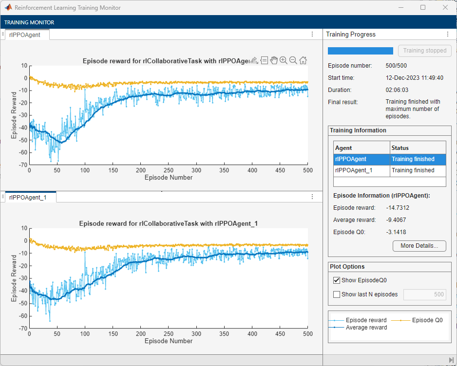
Train the agents using the train function. Training can take several hours to complete depending on the available computational power. To save time, load the MAT file decentralizedAgents.mat which contains a set of pretrained agents. To train the agents yourself, set dcTraining to true.
dcTraining =false; if dcTraining dcResults = train([dcAgentA,dcAgentB], env, dcOpts); else load("decentralizedAgents.mat"); end
The following figure shows a snapshot of decentralized training progress. You can expect different results due to randomness in the training process.
2. Centralized Training
Fix the random stream for reproducibility.
rng(0,"twister");To configure centralized multiagent training for this example:
Allocate both agents (with indices
1and2) in a single group. You can do this by specifying the agent indices in the"AgentGroups"option.Specify the
"centralized"learning strategy.Run the training for
500episodes, with each episode lasting a maximum of600time steps.
cnOpts = rlMultiAgentTrainingOptions( ...
    AgentGroups={[1,2]}, ...
    LearningStrategy="centralized", ...
    MaxEpisodes=500, ...
    MaxStepsPerEpisode=600, ...
    ScoreAveragingWindowLength=30, ...
    StopTrainingCriteria="none");
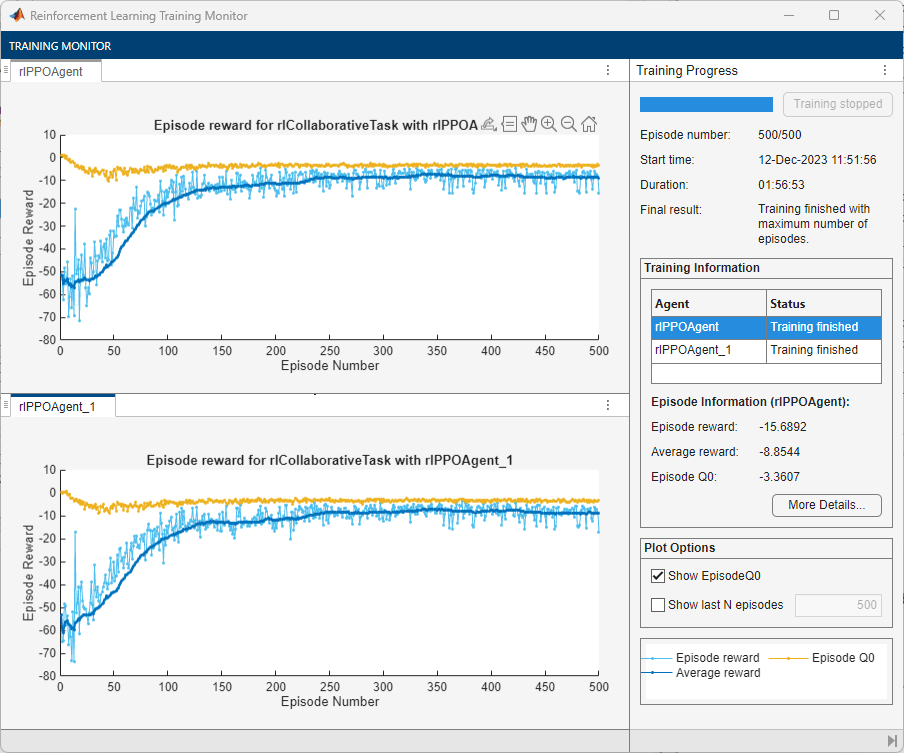
Train the agents using the train function. Training can take several hours to complete depending on the available computational power. To save time, load the MAT file centralizedAgents.mat which contains a set of pretrained agents. To train the agents yourself, set cnTraining to true.
cnTraining =false; if cnTraining cnResults = train([cnAgentA,cnAgentB], env, cnOpts); else load("centralizedAgents.mat"); end
The following figure shows a snapshot of centralized training progress. You can expect different results due to randomness in the training process.
Simulate Environment
Fix the random stream for reproducibility.
rng(0,"twister");Create a simulation options object to run the simulation with a maximum of 600 environment steps.
simOptions = rlSimulationOptions(MaxSteps=600);
Simulate the trained (decentralized) agents with the environment.
simulationChoice ="decentralized"; if strcmpi(simulationChoice,"decentralized") dcExp = sim(env,[dcAgentA,dcAgentB],simOptions); end
To simulate the trained centralized agents set simulationChoice to centralized.
if strcmpi(simulationChoice,"centralized")
    cnExp = sim(env,[cnAgentA,cnAgentB],simOptions);
end
The agents are able to push the object outside the ring.
For more information on agent simulation, see rlSimulationOptions and sim.
Restore the random number stream using the information stored in previousRngState.
rng(previousRngState);
Local Functions
The sim function calls the reset function at the start of each simulation episode, and the train function calls it at the start of each training episode. The reset function takes as input, and returns as output, a Simulink.SimulationInput (Simulink) object. The output object specifies temporary changes applied to model, which are then discarded when the simulation or training completes. For this example, the you use setVariable (Simulink) to set variables in the model workspace. For more information, see Reset Function for Simulink Environments.
function in = resetRobots(in,RA,RB,RC,boundaryR)
% Reset the environment.

% Random initial positions
valid = false;
while ~valid
    xA0 = -10 + 20*rand;
    yA0 = -10 + 20*rand;
    xB0 = -10 + 20*rand;
    yB0 = -10 + 20*rand;
    r = 0.5*boundaryR*rand;
    th = -pi + 2*pi*rand;
    xC0 = r*cos(th);
    yC0 = r*sin(th);
    dAB = norm([xA0-xB0;yA0-yB0]);
    dBC = norm([xB0-xC0;yB0-yC0]);
    dAC = norm([xA0-xC0;yA0-yC0]);
    dA = norm([xA0;yA0]);
    dB = norm([xB0;yB0]);
    valid = dA > boundaryR && ...
        dB > boundaryR && ...
        dAB > (RA+RB) && ...
        dBC > (RB+RC) && ...
        dAC > (RA+RC);
end

% Set the variables in the simulation input object
in = setVariable(in,'xA0',xA0);
in = setVariable(in,'xB0',xB0);
in = setVariable(in,'yA0',yA0);
in = setVariable(in,'yB0',yB0);
Main helper function to plot the environment.
% Set a post sim function for visualization
in = setPostSimFcn(in,@(out) localPostSim(out,RA,RB,RC,boundaryR));
end

function out = localPostSim(out,RA,RB,RC,boundaryR)
tsqA = localGetState(out,'qA');
tsqB = localGetState(out,'qB');
tsqC = localGetState(out,'qC');
xA = tsqA.Data(:,1);
xB = tsqB.Data(:,1);
xC = tsqC.Data(:,1);
yA = tsqA.Data(:,2);
yB = tsqB.Data(:,2);
yC = tsqC.Data(:,2);
t = tsqA.Time;
for i = 1:numel(xA)
    plotEnvironment( ...
        [xA(i);xB(i);xC(i)], ...
        [yA(i);yB(i);yC(i)], ...
        [RA;RB;RC], boundaryR, t(i));
    drawnow();
end
end

function ts = localGetState(out,name)
stateObj = out.logsout.get(name);
ts = stateObj.Values;
end
Secondary helper function to plot the environment (called from the setPostSimFcn).
function plotEnvironment(x,y,R,boundaryR,t)
% Plot the environment.

persistent f;
if isempty(f) || ~isvalid(f)
    f = figure( ...
        NumberTitle="off", ...
        Name="Multi Agent Collaborative Task", ...
        MenuBar="none", ...
        Position=[500,500,300,300], ...
        Visible="on");
    ha = gca(f);
    axis(ha,"equal");
    ha.XLim = [-12 12];
    ha.YLim = [-12 12];
    xlabel(ha,"X (m)");
    ylabel(ha,"Y (m)");

    D = [-1 -1 2 2]*boundaryR;
    rectangle(ha,Position=D,Curvature=[1 1]);

    hold(ha,'on');
end
% plot elements
ha = gca(f);
N = numel(R);
colors = ["r","g","b"];
for i = 1:N
    D = [(x(i)-R(i)) (y(i)-R(i)) 2*R(i) 2*R(i)];
    tagstr = sprintf("rect_%u",i);
    r = findobj(ha,Tag=tagstr);
    if isempty(r)
        r = rectangle(ha,Position=D,Curvature=[1 1],Tag=tagstr);
        r.FaceColor = colors(i);
    else
        r.Position = D;
    end
end
% Display time string
timestr = sprintf("Time: %0.1f s",t);
time = findobj(ha,Tag="time");
if isempty(time)
    text(ha,5,10,timestr,Tag="time");
else
    time.String = timestr;
end
end
See Also
Functions
train|sim|rlSimulinkEnv