Use Predefined Grid World Environments
Reinforcement Learning Toolbox™ software provides several predefined grid world environments for which the actions, observations, rewards, and dynamics are already defined. You can use these environments to:
Learn reinforcement learning concepts.
Gain familiarity with grid world environments and Reinforcement Learning Toolbox software features.
Test your own discrete-action-space reinforcement learning agents.
To create your own custom grid world environments instead, see Create Custom Grid World Environments.
To create an object that implements one of the following predefined MATLAB® grid world environments, use the rlPredefinedEnv
function. For example, at the MATLAB command line, type: env =
rlPredefinedEnv("BasicGridWorld").
| Environment | Agent Task |
|---|---|
| Basic Grid World | Move from a starting location to a target location on a two-dimensional grid by
selecting moves from the discrete action space {N,S,E,W}. |
| Deterministic Waterfall Grid World | Move from a starting location to a target location on a larger two-dimensional grid with unknown deterministic dynamics. |
| Stochastic Waterfall Grid World | Move from a starting location to a target location on a larger two-dimensional grid with unknown stochastic dynamics. |
Reinforcement Learning Toolbox implements these grid world environments as rlMDPEnv objects. For
more information on the properties of grid world environments, see Create Custom Grid World Environments.
You can also create objects that implement predefined MATLAB control system environments. For more information, see Use Predefined Control System Environments.
Basic Grid World
The basic grid world environment is a two-dimensional 5-by-5 grid with a starting location, a terminal location, and obstacles. The environment also contains a special jump from state [2,4] to state [4,4]. The goal of the agent is to move from the starting location to the terminal location while avoiding obstacles and maximizing the total reward.
To create a basic grid world environment, use the rlPredefinedEnv
function. When you use the keyword "BasicGridWorld" this function returns
an rlMDPEnv object
representing the grid world.
env =
      rlPredefinedEnv("BasicGridWorld")
env =

  rlMDPEnv with properties:

       Model: [1×1 rl.env.GridWorld]
    ResetFcn: []
Here, the Model property of env is a
GridWorld object that encodes all the environment properties including
its observation dynamics, the rewards returned to the agent for each move, and the possible
presence of obstacles and terminals states. For more information on
GridWorld objects, see Create Custom Grid World Environments.
You can use the ResetFcn property to specify your own reset
function, instead of the default function that returns a random state. A training or
simulation function automatically calls the reset function at the beginning of each training
or simulation episode. For more information on how to set the reset function of this
environment, see Reset Function.
For an example that compares discrete state space agents on this environment, see Compare Agents on Basic Grid World.
Environment Visualization
You can visualize the grid world environment using the plot
function.
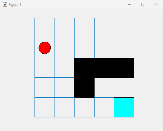
The agent location is a red circle. In this case, the agent location is [1,1], corresponding to the environment state number 1.
The terminal location is a light blue square.
The obstacles are black squares.
plot(env)

Note
Visualizing the environment during training can provide insight, but it tends to increase training time. For faster training, keep the environment plot closed during training.
Actions
For this environment, the action channel carries a scalar integer from 1 to 4 that
indicates an attempted move in one of four possible directions: north, south, east, or
west, respectively. Therefore the agent has an action channel which is specified by an
rlFiniteSetSpec
object. To extract the action specification, use the getActionInfo
function.
actInfo = getActionInfo(env)
actInfo =

  rlFiniteSetSpec with properties:

       Elements: [4×1 double]
           Name: "MDP Actions"
    Description: [0×0 string]
      Dimension: [1 1]
       DataType: "double"
Observations
The observation is composed by a single channel carrying a scalar integer from 1 to
25. This integer indicates the current agent location (that is, the environment state) in
column-wise fashion. For example, the observation 5 corresponds to the agent position
[5,1] on the grid, the observation 6 corresponds to the position [1,2], and so on.
Therefore the observation specification is an rlFiniteSetSpec
object. To extract the observation specification, use the getObservationInfo
function.
obsInfo = getObservationInfo(env)
obsInfo =

  rlFiniteSetSpec with properties:

       Elements: [25×1 double]
           Name: "MDP Observations"
    Description: [0×0 string]
      Dimension: [1 1]
       DataType: "double"
Dynamics
If the agent attempts an illegal move, such as an action that moves it out of the grid or into an obstacle, the resulting position of the agent remains unchanged, otherwise, the environment updates the position of the agent according to the action. For example, if the agent is in the position 5, the action 3 (an attempted move eastward) moves the agent to the position 10 at the next time step. The action 4 (an attempted move westward) instead results in the agent maintaining position 5 at the next time step.
You can customize the default dynamics by modifying the transition matrix, and the
number and position of the obstacle and terminal states in the underlying
GridWorld object. For more information, see Create Grid World Object.
Rewards
The action A(t) results in the transition from the current state S(t) to the following state S(t+1), which in turn results in these rewards or penalties from the environment to the agent, represented by the scalar R(t+1):
+10reward for reaching the terminal state at [5,5]+5reward for jumping from state [2,4] to state [4,4]-1penalty for every other action
You can customize the default rewards by modifying the reward matrix in the underlying
GridWorld object. For more information, see Create Grid World Object.
Reset Function
The default reset function for this environment sets the initial environment state randomly, while avoiding the obstacle and the target cells.
x0 = reset(env)
x0 =

    11
You can write your own reset function to specify a different initial state. For
example, to specify that the initial state of the environment (that is, the initial
position of the agent on the grid) is always 2, create a reset function that always
returns 2, and set the ResetFcn property to the
handle of the function.
env.ResetFcn = @() 2;
A training or simulation function automatically calls the reset function at the beginning of each training or simulation episode.
Create an Agent for This Environment
Using default agents for tabular problems is not recommended. This is because default agents rely on neural network approximation models for their actors an critics, and these model generally do not approximate tables satisfactorily, leading to poor overall performance.
In general Q, SARSA, and DQN agents that use a table-based critic perform well on tabular problems. For an example comparing discrete state space agents on this environment, see Compare Agents on Basic Grid World.
For more information on creating agents, see Reinforcement Learning Agents.
Step Function
You can also call the environment step function to return the next observation,
reward, and an is-done scalar indicating whether the environment
reaches a final state. For example, reset the basic grid world environment and call the
step function with an action input of 3 (move east).
First, reset the environment.
x0 = reset(env)
x0 =

     2
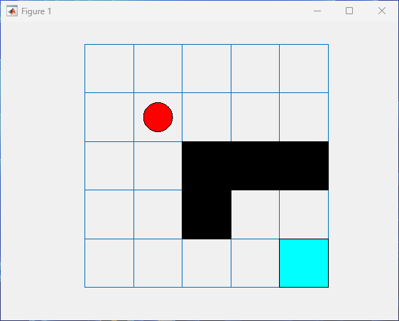
Visualize the environment.
plot(env)
Move the agent eastward.
[xn,rn,id]=step(env,3)
     7


rn =

    -1


id =

  logical

   0
After the step function executes, the environment plot, if present, visualizes the new position of the agent on the grid.
As described in the Observations and Rewards sections, an attempted move
either outside the grid or into a position where an obstacle is present results in the
agent staying in the same position, while still collecting a reward of
-1.
The environment step and reset functions
allow you to create a custom training or simulation loop. For more information on custom
training loops, see Train Reinforcement Learning Policy Using Custom Training Loop.
Environment Code
To access the function that returns this environment, at the MATLAB command line, type:
edit rl.env.BasicGridWorldDeterministic Waterfall Grid World
The deterministic waterfall grid world environment is a two-dimensional 8-by-7 grid with a starting location and a terminal location. The environment includes a waterfall that pushes the agent toward the bottom of the grid. The goal of the agent is to move from the starting location to the terminal location while maximizing the total reward.
To create a deterministic waterfall grid world, use the rlPredefinedEnv
function. This function creates an rlMDPEnv object
representing the grid world.
env = rlPredefinedEnv("WaterFallGridWorld-Deterministic")env =
rlMDPEnv with properties:
Model: [1×1 rl.env.GridWorld]
ResetFcn: []
Here, the Model property of env is a
GridWorld object that encodes all the environment properties including
its observation dynamics, the rewards returned to the agent for each move, and the possible
presence of obstacles and terminals states.
You can use the ResetFcn property to specify your own reset
function, instead of the default function that which returns a random state. The reset
function is called (by a training or simulation function) at the beginning of each training
or simulation episode. For more information on how to set the reset function of this
environment, see Reset Function.
For an example that compares discrete state space agents on this environment, see Compare Agents on Deterministic Waterfall Grid World.
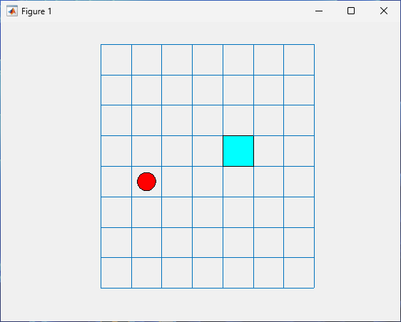
Environment Visualization
As with any grid world environment, you can visualize the environment using the
plot function.
plot(env)
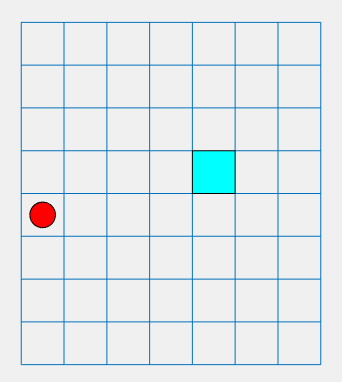
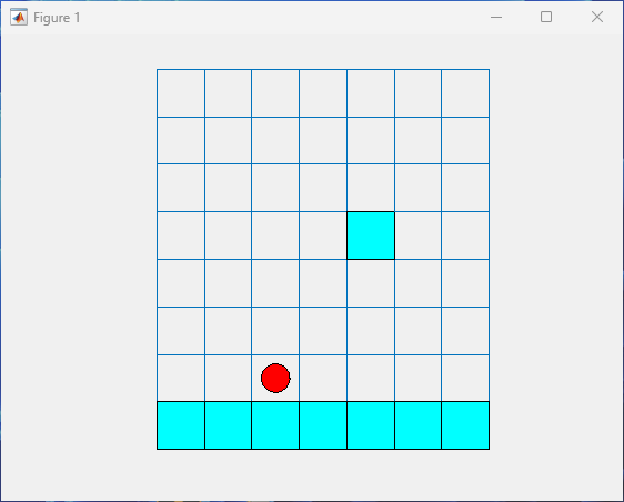
Here the agent position is represented with a red circle and the terminal location is represented with light blue squares.
Note
Visualizing the environment during training can provide insight, but it tends to increase training time. For faster training, keep the environment plot closed during training.
Actions
As in all other predefined grid world environments, in a deterministic waterfall
environment the action channel carries a scalar integer from 1 to 4, which indicates an
attempted move in one of four possible directions: north, south, east, or west,
respectively. Therefore, the action specification is an rlFiniteSetSpec
object. To extract the action specification, use the getActionInfo
function.
actInfo = getActionInfo(env)
actInfo =

  rlFiniteSetSpec with properties:

       Elements: [4×1 double]
           Name: "MDP Actions"
    Description: [0×0 string]
      Dimension: [1 1]
       DataType: "double"
Observations
The observation has a single channel carrying a scalar integer from 1 to 56. This
integer indicates the current agent location (that is, the environment state) in
columnwise fashion. For example, the observation 8 corresponds to the agent position [8,1]
on the grid, the observation 9 corresponds to the position [1,2], and so on. Therefore the
observation specification is an rlFiniteSetSpec
object. To extract the observation specification, use the getObservationInfo
function.
obsInfo = getObservationInfo(env)
obsInfo =

  rlFiniteSetSpec with properties:

       Elements: [56×1 double]
           Name: "MDP Observations"
    Description: [0×0 string]
      Dimension: [1 1]
       DataType: "double"
Dynamics
If the agent attempts an illegal move, such as an action that moves it out of the grid, the resulting position remains unchanged, otherwise, the environment updates the agent position according to the action. For example, if the agent is in the position 8, the action 3 (an attempted move eastward) moves the agent to the position 10 at the next time step. The action 4 (an attempted move westward) results in the agent maintaining the position 8 at the next time step.
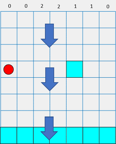
In a deterministic waterfall grid world environment, a waterfall pushes the agent toward the bottom of the grid.
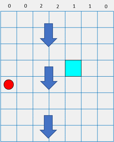
The intensity of the waterfall varies between the columns, as shown at the top of the figure. When the agent moves into a column with a nonzero intensity, the waterfall pushes it downward by the indicated number of squares. For example, if the agent attempts to move east from the position [5,2] (environment state number 13), it reaches position [7,3] (environment state number 23).
You can customize the default dynamics by modifying the transition matrix, and the
number and position of the obstacle and terminal states in the underlying
GridWorld object. For more information, see Create Grid World Object.
Rewards
The action A(t) results in the transition from the current state S(t) to the following state S(t+1), which in turn results in these rewards or penalties from the environment to the agent, represented by the scalar R(t+1):
+10reward for reaching the terminal position at [4,5]-1penalty for every other action
You can customize the default rewards by modifying the reward matrix in the underlying
GridWorld object. For more information, see Create Grid World Object.
Reset Function
The default reset function for this environment sets the initial environment state (that is, the initial position of the agent on the grid) randomly, while avoiding the target cell.
x0 = reset(env)
x0 =

    12
You can write your own reset function to specify a different initial state. For
example, to specify that the initial state of the environment is always 5, create a reset
function that always returns 5, and set the
ResetFcn property to the handle of the function.
env.ResetFcn = @() 5;
A training or simulation function automatically calls the reset function at the beginning of each training or simulation episode.
Create an Agent for This Environment
Using default agents for tabular problems is not recommended. This is because default agents rely on neural network approximation models for their actors an critics, and these model generally do not approximate tables satisfactorily, leading to poor overall performance.
In general Q, SARSA, and DQN agents that use a table-based critic perform well on tabular problems. For an example comparing discrete state space agents on this environment, see Compare Agents on Deterministic Waterfall Grid World.
For more information on creating agents, see Reinforcement Learning Agents.
Step Function
The environment observation and action specifications allow you to create an agent
that works with your environment. You can then use both the environment and agent as
arguments for the built-in functions train and
sim, which train
or simulate the agent within the environment, respectively.
You can also call the environment step function to return the next observation, reward
and an is-done scalar indicating whether the environment reaches a
final state.
For example, first define a reset function so that the initial position of the agent on the grid is always [5,2], encoded by the environment state number 13.
env.ResetFcn = @() 13;
Reset the environment.
reset(env)
ans =

    13
Plot the environment.
plot(env)
Call the step function with an action input of 3 (move
east).
[xn,rn,id]=step(env,3)
xn =

    23


rn =

    -1


id =

  logical

   0
The environment plot visualizes the new position of the agent on the grid.
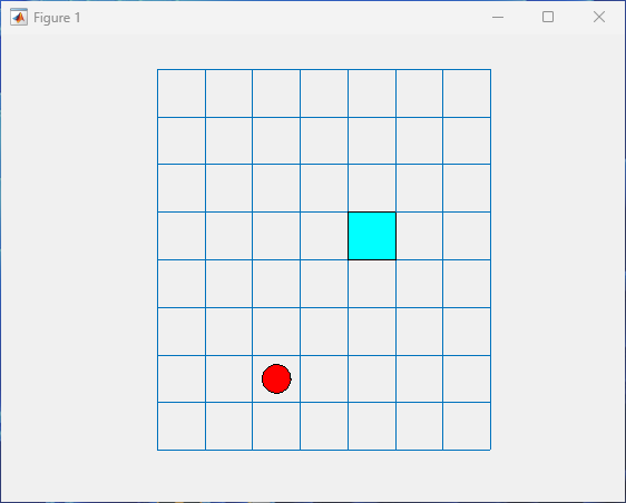
Due to the downward waterfall, the agent moves considerably southward to the position [5,3], directly east from the position [5,2].
The environment step and reset functions
allow you to create a custom training or simulation loop. For more information on custom
training loops, see Train Reinforcement Learning Policy Using Custom Training Loop.
Environment Code
To access the function that returns this environment, at the MATLAB command line, type:
edit rl.env.WaterFallDeterministicGridWorldStochastic Waterfall Grid World
The stochastic waterfall grid world environment is a two-dimensional 8-by-7 grid with a starting location and eight terminal locations. The environment includes a waterfall that pushes the agent toward the bottom of the grid with a stochastic intensity. The goal of the agent is to move from the starting location to the target terminal location while avoiding the penalty terminal states along the bottom of the grid and maximizing the total reward.
To create a stochastic waterfall grid world, use the rlPredefinedEnv
function. This function creates an rlMDPEnv object
representing the grid world.
env = rlPredefinedEnv("WaterFallGridWorld-Stochastic");env =
rlMDPEnv with properties:
Model: [1×1 rl.env.GridWorld]
ResetFcn: []
Here, the Model property of env is a
GridWorld object that encodes all the environment properties including
its observation dynamics, the rewards returned to the agent for each move, and the possible
presence of obstacles and terminals states. For more information on
GridWorld objects, see Create Custom Grid World Environments.
You can use the ResetFcn property to specify your own reset
function, instead of the default one (which returns a random state). A training or
simulation function automatically calls the reset function at the beginning of each training
or simulation episode. For more information on how to set the reset function of this
environment, see Reset Function.
For an example comparing discrete state space agents on this environment, see Compare Agents on Stochastic Waterfall Grid World.
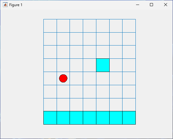
Environment Visualization
As with any grid world environment, you can visualize the environment using the
plot function.
plot(env)

Here the agent position is represented with a red circle and the terminal locations are represented with light blue squares.
Note
Visualizing the environment during training can provide insight, but it tends to increase training time. For faster training, keep the environment plot closed during training.
Actions
As in all predefined grid world environments, in a stochastic waterfall environment
the action channel carries a scalar integer from 1 to 4 that indicates an attempted move
in one of four possible directions: north, south, east, or west, respectively. Therefore,
the action specification is an rlFiniteSetSpec
object. To extract the action specification, use the getActionInfo
function.
actInfo = getActionInfo(env)
actInfo =

  rlFiniteSetSpec with properties:

       Elements: [4×1 double]
           Name: "MDP Actions"
    Description: [0×0 string]
      Dimension: [1 1]
       DataType: "double"
Observations
The observation has a single channel carrying a scalar integer from 1 to 56. This
integer indicates the current agent location (that is, the environment state) in
columnwise fashion. For example, the observation 8 corresponds to the agent position [8,1]
on the grid, the observation 9 corresponds to the position [1,2], and so on. Therefore the
observation specification is an rlFiniteSetSpec
object. To extract the observation specification, use the getObservationInfo
function.
obsInfo = getObservationInfo(env)
obsInfo =

  rlFiniteSetSpec with properties:

       Elements: [56×1 double]
           Name: "MDP Observations"
    Description: [0×0 string]
      Dimension: [1 1]
       DataType: "double"
Dynamics
If the agent attempts an illegal move, such as an action that moves the agent out of the grid, the resulting position remains unchanged, otherwise, the environment updates the agent position according to the action. For example, if the agent is in the position 8, the action 3 (an attempted move eastward) moves the agent to the position 10 at the next time step. The action 4 (an attempted move westward) results in the agent still keeping position 8 at the next time step.
In a stochastic waterfall grid world, a waterfall pushes the agent toward the bottom of the grid with a stochastic intensity.
The baseline intensity matches the intensity of the deterministic waterfall environment. However, in the stochastic waterfall environment, the agent has an equal chance of experiencing the indicated intensity, one level above that intensity, or one level below that intensity. For example, if the agent moves east from state [5,2], it has an equal chance of reaching state [6,3], [7,3], or [8,3].
You can customize the default dynamics by modifying the transition matrix and the
number and position of the obstacle and terminal states in the underlying
GridWorld object. For more information, see Create Grid World Object.
Rewards
The action A(t) results in the transition from the current state S(t) to the following state S(t+1), which in turn results in these rewards or penalties from the environment to the agent, represented by the scalar R(t+1):
+10reward for reaching the terminal state at [4,5]-10penalty for reaching any terminal state in the bottom row of the grid-1penalty for every other action
You can customize the default rewards by modifying the reward matrix in the underlying
GridWorld object. For more information, see Create Grid World Object.
Reset Function
The default reset function for this environment sets the initial environment state (that is, the initial position of the agent on the grid) randomly, while avoiding the target cells.
x0 = reset(env)
x0 =

    12
You can write your own reset function to specify a different initial state. For
example, to specify that the initial state of the environment is always 5, create a reset
function that always returns 5, and set the
ResetFcn property to the handle of the function.
env.ResetFcn = @() 5;
A training or simulation function automatically calls the reset function at the beginning of each training or simulation episode.
Create an Agent for This Environment
Using default agents for tabular problems is not recommended. This is because default agents rely on neural network approximation models for their actors an critics, and these model generally do not approximate tables satisfactorily, leading to poor overall performance.
In general Q, SARSA, and DQN agents that use a table-based critic perform well on tabular problems. For an example comparing discrete state space agents on this environment, see Compare Agents on Stochastic Waterfall Grid World.
For more information on creating agents, see Reinforcement Learning Agents.
Step Function
You can also call the environment step function to return the next observation,
reward, and an is-done scalar indicating whether the environment
reaches a final state.
For example, first define a reset function so that the initial position of the agent on the grid is always [5,2], encoded by the environment state number 13.
env.ResetFcn = @() 13;
Reset the environment.
reset(env)
ans =

    13
Plot the environment.
plot(env)
Call the step function with an action input of 3 (move
east).
[xn,rn,id]=step(env,3)
xn =

    23


rn =

    -1


id =

  logical

   0
The environment plot visualizes the new position of the agent on the grid.
Due to the downward waterfall, the agent moves considerably southward to the position [5,3], directly east from the position [5,2].
The environment step and reset functions
allow you to create a custom training or simulation loop. For more information on custom
training loops, see Train Reinforcement Learning Policy Using Custom Training Loop.
Environment Code
To access the function that returns this environment, at the MATLAB command line, type:
edit rl.env.WaterFallStochasticGridWorld