Automatic Target Recognition (ATR) in SAR Images
This example shows how to train a region-based convolutional neural network (R-CNN) for target recognition in large-scene synthetic aperture radar (SAR) images using Deep Learning Toolbox™ and Parallel Computing Toolbox™.
Deep Learning Toolbox provides a framework for designing and implementing deep neural networks with algorithms, pretrained models, and apps.
Parallel Computing Toolbox lets you solve computationally and data-intensive problems using multicore processors, GPUs, and computer clusters. It enables you to use GPUs directly from MATLAB® and accelerate the computation capabilities needed in deep learning algorithms.
Neural network based algorithms have shown remarkable achievement in diverse areas ranging from natural scene detection to medical imaging. They have shown huge improvement over the standard detection algorithms. Inspired by these advancements, researchers have put efforts to apply deep learning based solutions to the field of SAR imaging. In this example, the solution has been applied to solve the problem of target detection and recognition. The R-CNN network employed here not only solves problem of integrating detection and recognition but also provides an effective and efficient performance solution that scales to large scene SAR images as well.
This example demonstrates how to:
Download the dataset and the pretrained model
Load and analyze the image data
Define the network architecture
Specify training options
Train the network
Evaluate the network
To illustrate this workflow, the example uses the Moving and Stationary Target Acquisition and Recognition (MSTAR) clutter dataset published by the Air Force Research Laboratory. The dataset is available for download here. Alternatively, the example also includes a subset of the data used to showcase the workflow. The goal is to develop a model that can detect and recognize the targets.
Download the Dataset
This example uses a subset of the MSTAR clutter dataset that contains 300 training and 50 testing clutter images with five different targets. The data was collected using an X-band sensor in the spotlight mode with a one-foot resolution. The data contains rural and urban types of clutters. The types of targets used are BTR-60 (armoured car), BRDM-2 (fighting vehicle), ZSU-23/4 (tank), T62 (tank), and SLICY (multiple simple geometric shaped static target). The images were captured at a depression angle of 15 degrees. The clutter data is stored in the PNG image format and the corresponding ground truth data is stored in the groundTruthMSTARClutterDataset.mat file. The file contains 2-D bounding box information for five classes, which are SLICY, BTR-60, BRDM-2, ZSU-23/4, and T62 for training and testing data. The size of the dataset is 1.6 GB.
Download the dataset using the helperDownloadMSTARClutterData helper function, defined at the end of this example.
outputFolder = pwd;
dataURL = ('https://ssd.mathworks.com/supportfiles/radar/data/MSTAR_ClutterDataset.tar.gz');
helperDownloadMSTARClutterData(outputFolder,dataURL);
Depending on your Internet connection, the download process can take some time. The code suspends MATLAB® execution until the download process is complete. Alternatively, download the dataset to a local disk using your web browser and extract the file. When using this approach, change the <outputFolder> variable in the example to the location of the downloaded file.
Download the Pretrained Network
Download the pretrained network from the link here using the helperDownloadPretrainedSARDetectorNet helper function, defined at the end of this example. The pretrained model allows you to run the entire example without having to wait for the training to complete. To train the network, set the doTrain variable to true.
pretrainedNetURL = ('https://ssd.mathworks.com/supportfiles/radar/data/TrainedSARDetectorNet.tar.gz'); doTrain =false; if ~doTrain helperDownloadPretrainedSARDetectorNet(outputFolder,pretrainedNetURL); end
Load the Dataset
Load the ground truth data (training set and test set). These images are generated in such a way that it places target chips at random locations on a background clutter image. The clutter image is constructed from the downloaded raw data. The generated target will be used as ground truth targets to train and test the network.
load('groundTruthMSTARClutterDataset.mat', "trainingData", "testData");
The ground truth data is stored in a six-column table, where the first column contains the image file paths and the second to the sixth columns contain the different target bounding boxes.
% Display the first few rows of the data set
trainingData(1:4,:)ans=4×6 table
imageFilename SLICY BTR_60 BRDM_2 ZSU_23_4 T62
______________________________ __________________ __________________ __________________ ___________________ ___________________
"./TrainingImages/Img0001.png" {[ 285 468 28 28]} {[ 135 331 65 65]} {[ 597 739 65 65]} {[ 810 1107 80 80]} {[1228 1089 87 87]}
"./TrainingImages/Img0002.png" {[595 1585 28 28]} {[ 880 162 65 65]} {[308 1683 65 65]} {[1275 1098 80 80]} {[1274 1099 87 87]}
"./TrainingImages/Img0003.png" {[200 1140 28 28]} {[961 1055 65 65]} {[306 1256 65 65]} {[ 661 1412 80 80]} {[ 699 886 87 87]}
"./TrainingImages/Img0004.png" {[ 623 186 28 28]} {[ 536 946 65 65]} {[ 131 245 65 65]} {[1030 1266 80 80]} {[ 151 924 87 87]}
Display one of the training images and box labels to visualize the data.
img = imread(trainingData.imageFilename(1));
bbox = reshape(cell2mat(trainingData{1,2:end}),[4,5])';
labels = {'SLICY', 'BTR_60', 'BRDM_2',  'ZSU_23_4', 'T62'};
annotatedImage = insertObjectAnnotation(img,'rectangle',bbox,labels,...
    'TextBoxOpacity',0.9,'FontSize',50);
figure
imshow(annotatedImage);
title('Sample Training Image With Bounding Boxes and Labels')
Define the Network Architecture
Create an R-CNN object detector for five targets: SLICY, BTR_60, BRDM_2, ZSU_23_4, T62.
objectClasses = {'SLICY', 'BTR_60', 'BRDM_2', 'ZSU_23_4', 'T62'};The network must be able to classify the five targets and a background class in order to be trained using the trainRCNNObjectDetector function available in Deep Learning Toolbox™. 1 is added in the code below to include the background class.
numClassesPlusBackground = numel(objectClasses) + 1;
The final fully connected layer of the network defines the number of classes that it can classify. Set the final fully connected layer to have an output size equal to numClassesPlusBackground.
% Define input size
inputSize = [128,128,1];

% Define network
layers = createNetwork(inputSize,numClassesPlusBackground);
Now, these network layers can be used to train an R-CNN based five-class object detector.
Train Faster R-CNN
Use trainingOptions (Deep Learning Toolbox) to specify network training options. trainingOptions by default uses a GPU if one is available (requires Parallel Computing Toolbox™ and a CUDA® enabled GPU with compute capability 3.0 or higher). Otherwise, it uses a CPU. You can also specify the execution environment by using the ExecutionEnvironment name-value argument of trainingOptions. To detect automatically if you have a GPU available, set ExecutionEnvironment to auto. If you do not have a GPU, or do not want to use one for training, set ExecutionEnvironment to cpu. To ensure the use of a GPU for training, set ExecutionEnvironment to gpu.
% Set training options
options = trainingOptions('sgdm', ...
    'MiniBatchSize', 128, ...
    'InitialLearnRate', 1e-3, ...
    'LearnRateSchedule', 'piecewise', ...
    'LearnRateDropFactor', 0.1, ...
    'LearnRateDropPeriod', 100, ...
    'MaxEpochs', 10, ...
    'Verbose', true, ...
    'CheckpointPath',tempdir,...
    'ExecutionEnvironment','auto');
Use trainRCNNObjectDetector to train R-CNN object detector if doTrain is true. Otherwise, load the pretrained network. If training, adjust NegativeOverlapRange and PositiveOverlapRange to ensure that training samples tightly overlap with ground truth.
if doTrain
    % Train an R-CNN object detector. This will take several minutes
    detector = trainRCNNObjectDetector(trainingData, layers, options,'PositiveOverlapRange',[0.5 1], 'NegativeOverlapRange', [0.1 0.5]);
else
    % Load a previously trained detector
    preTrainedMATFile = fullfile(outputFolder,'TrainedSARDetectorNet.mat');
    load(preTrainedMATFile);
end
Evaluate Detector on a Test Image
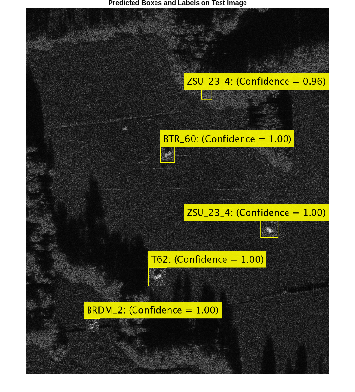
To get a qualitative idea of the functioning of the detector, pick a random image from the test set and run it through the detector. The detector is expected to return a collection of bounding boxes where it thinks the detected targets are, along with scores indicating confidence in each detection.
% Read test image
imgIdx = randi(height(testData));
testImage = imread(testData.imageFilename(imgIdx));

% Detect SAR targets in the test image
[bboxes,score,label] = detect(detector,testImage,'MiniBatchSize',16);
To understand the results achieved, overlay the results with the test image. A key parameter is the detection threshold, the score above which the detector detected a target. A higher threshold will result in fewer false positives; however, it also results in more false negatives.
scoreThreshold =0.8; % Display the detection results outputImage = testImage; for idx = 1:length(score) bbox = bboxes(idx, :); thisScore = score(idx); if thisScore > scoreThreshold annotation = sprintf('%s: (Confidence = %0.2f)', label(idx),... round(thisScore,2)); outputImage = insertObjectAnnotation(outputImage, 'rectangle', bbox,... annotation,'TextBoxOpacity',0.9,'FontSize',45,'LineWidth',2); end end f = figure; f.Position(3:4) = [860,740]; imshow(outputImage) title('Predicted Boxes and Labels on Test Image')
Evaluate Model
By looking at the images sequentially, you can understand the detector performance. To perform more rigorous analysis using the entire test set, run the test set through the detector.
% Create a table to hold the bounding boxes, scores and labels output by the detector
numImages = height(testData);
results = table('Size',[numImages 3],...
    'VariableTypes',{'cell','cell','cell'},...
    'VariableNames',{'Boxes','Scores','Labels'});

% Run detector on each image in the test set and collect results
for i = 1:numImages
    imgFilename = testData.imageFilename{i};

    % Read the image
    I = imread(imgFilename);

    % Run the detector
    [bboxes, scores, labels] = detect(detector, I,'MiniBatchSize',16);

    % Collect the results
    results.Boxes{i} = bboxes;
    results.Scores{i} = scores;
    results.Labels{i} = labels;
end
The possible detections and their bounding boxes for all images in the test set can be used to calculate the detector's average precision (AP) for each class. The AP is the average of the detector's precision at different levels of recall, so let us define precision and recall.
where
- Number of true positives (the detector predicts a target when it is present)
- Number of false positives (the detector predicts a target when it is not present)
- Number of false negatives (the detector fails to detect a target when it is present)
A detector with a precision of 1 is considered good at detecting targets that are present, while a detector with a recall of 1 is good at avoiding false detections. Precision and recall have an inverse relationship.
Plot the relationship between precision and recall for each class. The average value of each curve is the AP. Plot curves for detection thresholds with the value of 0.5.
For more details, see evaluateObjectDetection (Computer Vision Toolbox).
% Format test data as a combined datastore
imds = imageDatastore(testData.imageFilename);
blds = boxLabelDatastore(testData(:,2:end));
cds  = combine(imds,blds); % CombinedDatastore

% Evaluate the object detector using average precision metric
metrics   = evaluateObjectDetection(results,cds);
ap        = metrics.ClassMetrics.AP;
precision = metrics.ClassMetrics.Precision;
recall    = metrics.ClassMetrics.Recall;

% Plot precision recall curve
f = figure; ax = gca; f.Position(3:4) = [860,740];
xlabel('Recall')
ylabel('Precision')
grid on; hold on; legend('Location', 'southeast');
title('Precision Versus Recall');
for i = 1:length(ap)
    plot(ax,recall{i},precision{i},'DisplayName',['Average Precision for Class ' trainingData.Properties.VariableNames{i+1} ' is ' num2str(round(ap{i},3))])
end

The AP for most of the classes is excellent and is generally about 0.9 or better. Out of these, the trained model appears to struggle the most in detecting the SLICY targets. However, it is still able to achieve an AP of about 0.7 for the class.
Helper Function
The function createNetwork takes as input the image size inputSize and number of classes numClassesPlusBackground. The function returns a CNN.
function layers = createNetwork(inputSize,numClassesPlusBackground)
    layers = [
        imageInputLayer(inputSize)                      % Input Layer
        convolution2dLayer(3,32,'Padding','same')       % Convolution Layer
        reluLayer                                       % Relu Layer
        convolution2dLayer(3,32,'Padding','same')
        batchNormalizationLayer                         % Batch normalization Layer
        reluLayer
        maxPooling2dLayer(2,'Stride',2)                 % Max Pooling Layer

        convolution2dLayer(3,64,'Padding','same')
        reluLayer
        convolution2dLayer(3,64,'Padding','same')
        batchNormalizationLayer
        reluLayer
        maxPooling2dLayer(2,'Stride',2)

        convolution2dLayer(3,128,'Padding','same')
        reluLayer
        convolution2dLayer(3,128,'Padding','same')
        batchNormalizationLayer
        reluLayer
        maxPooling2dLayer(2,'Stride',2)

        convolution2dLayer(3,256,'Padding','same')
        reluLayer
        convolution2dLayer(3,256,'Padding','same')
        batchNormalizationLayer
        reluLayer
        maxPooling2dLayer(2,'Stride',2)

        convolution2dLayer(6,512)
        reluLayer

        dropoutLayer(0.5)                               % Dropout Layer
        fullyConnectedLayer(512)                        % Fully connected Layer.
        reluLayer
        fullyConnectedLayer(numClassesPlusBackground)
        softmaxLayer                                    % Softmax Layer
        classificationLayer                             % Classification Layer
        ];

end

function helperDownloadMSTARClutterData(outputFolder,DataURL)
% Download the data set from the given URL to the output folder.

    radarDataTarFile = fullfile(outputFolder,'MSTAR_ClutterDataset.tar.gz');

    if ~exist(radarDataTarFile,'file')

        disp('Downloading MSTAR Clutter data (1.6 GB)...');
        websave(radarDataTarFile,DataURL);
        untar(radarDataTarFile,outputFolder);
    end
end

function helperDownloadPretrainedSARDetectorNet(outputFolder,pretrainedNetURL)
% Download the pretrained network.

    preTrainedMATFile = fullfile(outputFolder,'TrainedSARDetectorNet.mat');
    preTrainedZipFile = fullfile(outputFolder,'TrainedSARDetectorNet.tar.gz');

    if ~exist(preTrainedMATFile,'file')
        if ~exist(preTrainedZipFile,'file')
            disp('Downloading pretrained detector (29.4 MB)...');
            websave(preTrainedZipFile,pretrainedNetURL);
        end
        untar(preTrainedZipFile,outputFolder);
    end
end
Summary
This example shows how to train an R-CNN for target recognition in SAR images. The pretrained network attained an accuracy of more than 0.9.
References
MSTAR Overview. https://www.sdms.afrl.af.mil/index.php?collection=mstar
You can also select a web site from the following list:
Americas
- América Latina (Español)
- Canada (English)
- United States (English)
Europe
- Belgium (English)
- Denmark (English)
- Deutschland (Deutsch)
- España (Español)
- Finland (English)
- France (Français)
- Ireland (English)
- Italia (Italiano)
- Luxembourg (English)
- Netherlands (English)
- Norway (English)
- Österreich (Deutsch)
- Portugal (English)
- Sweden (English)
- Switzerland
- United Kingdom (English)