Radar Vertical Coverage over Terrain
The propagation path of a radar system is modified by the environment in which it operates. When overlooking a surface, the free space radiation pattern is modified by the reflected wave, which results in an interference pattern with lobes and nulls. In a lobe maximum, a radar return can increase by as much as 12 dB, whereas in a minimum the return can theoretically go to 0 dB.
The vertical coverage pattern is a detection contour. It offers a look into the performance of a radar system at a constant signal level as specified by the free space range. The vertical coverage considers the interference between the direct and ground-reflected rays, as well as refraction. This example defines an L-band radar system in the presence of heavy clutter and shows you how to visualize its three-dimensional vertical coverage over terrain.
Define the Radar
To start, specify an L-band surveillance radar with the following parameters:
Peak power: 3 kW
Operating frequency: 1 GHz
Transmit and receive antenna beamwidth: 20 degrees in azimuth and elevation
Pulse width: 2 μs
% Radar parameters
rfs        = 50e3;           % Free-space range (m)
rdrppower  = 3e3;            % Peak power (W)
fc         = 1e9;            % Operating frequency (Hz)
hpbw       = 20;             % Half-power beamwidth (deg)
rdrpulsew  = 2e-6;           % Pulse width (s)
tiltAng    = 1;              % Radar tilt (elevation) angle (deg)
azRotation = 80;             % Radar azimuth rotation angle (deg)

% Vertical coverage parameters
minEl      = 0;              % Minimum vertical coverage angle (deg)
maxEl      = 90;             % Maximum vertical coverage angle (deg)
elStepSize = 1;              % Elevation step size (deg)
azAng      = -60:2:60;       % Azimuth angles for elevation cuts (deg)
Convert the transmit antenna's half-power beamwidth (HPBW) values to gain using the beamwidth2gain function. Assume a cosine rectangular aperture, which is a good approximation for a real-world antenna.
rdrgain = beamwidth2gain(hpbw,"CosineRectangular"); % Transmit and receive antenna gain (dB)
Define Location
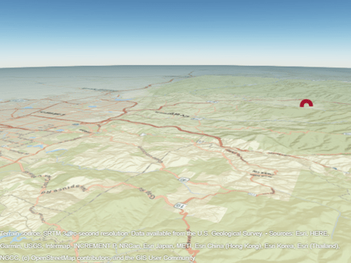
The next section defines the radar location. The radar is mounted on a tall tower 100 meters above the ground. The radar altitude is the sum of the ground elevation and the radar tower height referenced to the mean sea level (MSL). Visualize the location using geoplot3. The radar will appear as a red circular point in the upper right-hand corner of the image.
% Radar location
rdrlat = 39.5;           % Radar latitude (deg)
rdrlon = -105.5;         % Radar longitude (deg)
rdrtowerht = 100;        % Antenna height (m)
surfaceHtAtRadar = 2812; % Surface height at radar location (m)
rdralt = surfaceHtAtRadar + rdrtowerht; % Radar altitude (m)

% Import the relevant terrain data from the United States Geological
% Survey (USGS)
dtedfile = "n39_w106_3arc_v2.dt1";
attribution = "SRTM 3 arc-second resolution. Data available from the U.S. Geological Survey.";
[Z,R] = readgeoraster(dtedfile,OutputType="double");

% Visualize the location including terrain using the geographic globe plot
addCustomTerrain("southboulder",dtedfile,Attribution=attribution);

hTerrain = uifigure;

g = geoglobe(hTerrain,Terrain="southboulder",Basemap="streets");
hold(g,"on")
h_rdrtraj = geoplot3(g,rdrlat,rdrlon,rdralt,"o", ...
    Color=[0.6350 0.0780 0.1840],LineWidth=6,MarkerSize=6);

campos(g,40.0194565714502,-105.564712896622,13117.1497971643);
camheading(g,150.8665488888147);
campitch(g,-16.023558618352187);

Investigate Free Space Range
For this example, the free space range rfs is the range at which a target has the specified signal-to-noise ratio (SNR). Assume a large target with a 10 dBsm radar cross section (RCS). At this range, the free space target SNR can be calculated as follows.
trcs = db2pow(10); % RCS (m^2)
lambda = freq2wavelen(fc); % Wavelength (m)
tsnr = radareqsnr(lambda,rfs,rdrppower,rdrpulsew, ...
    "RCS",trcs,"Gain",rdrgain)
tsnr =
-0.7449
For our surveillance radar, the desired performance index is a probability of detection (Pd) of 0.8 and probability of false alarm (Pfa) below 1e-3. To make the radar system design more feasible, you can use a pulse integration technique to reduce the required SNR. For this system, assume noncoherent integration of 64 pulses. A good approximation of the minimum SNR needed for a detection at the specified Pd and Pfa can be computed by the detectability function as follows. Note that the free space SNR satisfies the detectability requirement.
Pd = 0.8;
Pfa = 1e-3;
minsnr = detectability(Pd,Pfa,64);
isdetectable = tsnr >= minsnr
isdetectable = logical
   1
The toccgh function allows you to translate receiver detection probabilities into track probabilities. Assuming the default tracker, the required Pd and Pfa translate to the following probability of target track (Pdt) and probability of false track (Pft).
[Pdt,Pft] = toccgh(Pd,Pfa)
Pdt =
0.9608
Pft =
1.0405e-06
The Pd and Pfa requirements enable a track probability of about 96% and a false track probability on the order of 1e-6.
Plot Vertical Coverage
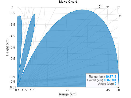
The vertical coverage pattern is visualized using a Blake chart, also known as a range-height-angle chart. The range along the x-axis is the propagated range and the height along the y-axis is relative to the origin of the ray.
The vertical coverage contour is calculated using the radarvcd function. The default permittivity model in radarvcd is based on a sea surface. Such a model is not applicable for the defined scenario, which is over land. Thus, the first step in simulating more realistic propagation is to select a more appropriate permittivity. Use the earthSurfacePermittivity function with the vegetation flag. Assume an ambient temperature of 21.1 degrees Celsius, which is about 70 degrees Fahrenheit. Assume a gravimetric water content of 0.3.
temp = 21.1; % Ambient temperature (degrees Celsius)
gwc = 0.3; % Gravimetric water content
[~,~,epsc] = earthSurfacePermittivity("vegetation",fc,temp,gwc);
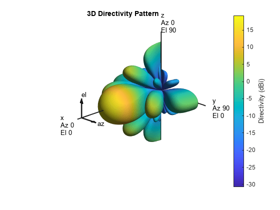
Next, specify the antenna. Simulate the antenna as a theoretical sinc antenna pattern and plot.
hBeam = phased.SincAntennaElement(Beamwidth=hpbw);
pattern(hBeam,fc);

Get the elevation pattern at 0 degrees azimuth by using the helperGetVoltagePattern function.
elAng = -90:0.01:90;
pat = helperGetVoltagePattern(hBeam,fc,0,elAng);
Specify the atmosphere and calculate the corresponding effective Earth radius. Since the latitude of the radar in this example is 39.5 degrees, a mid-latitude atmosphere model would be most appropriate. Assume that the time period is during the summer.
% Set effective Earth radius using the mid latitude atmosphere model
% in summer
[nidx,N] = refractiveidx([0 1e3],LatitudeModel="Mid",Season="Summer");
RGradient = (nidx(2) - nidx(1))/1e3;
Re = effearthradius(RGradient); % m
Next, calculate the vertical coverage pattern using the radarvcd function.
[vcpkm,vcpang] = radarvcd(fc,rfs.*1e-3,rdrtowerht, ...
    SurfaceRelativePermittivity=epsc, ...
    SurfaceHeightStandardDeviation=30, ...
    Vegetation="Trees", ...
    AntennaPattern=pat,PatternAngles=elAng, ...
    TiltAngle=tiltAng, ...
    EffectiveEarthRadius=Re, ...
    MinElevation=minEl, ...
    ElevationStepSize=elStepSize, ...
    MaxElevation=maxEl);
Use the surface height at the site to obtain the surface refractivity from refractiveidx.
% Calculate an appropriate surface
[~,Ns] = refractiveidx(surfaceHtAtRadar,LatitudeModel="Mid",Season="Summer");
Plot the vertical coverage using the blakechart function. The blakechart axes are formed using the Central Radio Propagation Laboratory (CRPL) reference atmosphere. The CRPL model is widely used and models the refractivity profile as an exponential decay versus height, which has been shown to be an excellent approximation for a normal atmosphere (an atmosphere that is not undergoing anomalous propagation like ducting). The CRPL model is tailored by setting the surface height refractivity and the refraction exponent to a value that is appropriate for the location in which the system is operating and the time of year.
Update the surface refractivity and the refraction exponent inputs in the function call. In the subsequent plot, the constant-signal-level of the contour is given by the previously calculated target SNR.
rexp = refractionexp(Ns);
blakechart(vcpkm,vcpang,ScalePower=1,SurfaceRefractivity=Ns,RefractionExponent=rexp)

Visualize 3-D Vertical Coverage over Terrain
The next section calculates the vertical coverage at the specified azimuth intervals. The vertical coverage range and angle is converted to height using the range2height function using the CRPL method. The range-height-angle values are then converted to Cartesian.
% Initialize Cartesian X, Y, Z outputs
numAz = numel(azAng);
numRows = numel(minEl:elStepSize:maxEl)+1;
vcpX = zeros(numRows,numAz);
vcpY = zeros(numRows,numAz);
vcpZ = zeros(numRows,numAz);
wgs84 = wgs84Ellipsoid;

% Obtain vertical coverage contour in Cartesian coordinates
for idx = 1:numAz
    % Get elevation pattern at this azimuth
    pat = helperGetVoltagePattern(hBeam,fc,azAng(idx),elAng);

    % Get terrain height information
    [xdir,ydir,zdir] = sph2cart(deg2rad(azAng(idx)+azRotation),0,1e3);
    [xlat,ylon,zlon] = enu2geodetic(xdir,ydir,zdir,rdrlat,rdrlon,rdralt,wgs84);
    [~,~,~,htsurf] = los2(Z,R,rdrlat,rdrlon, ...
        xlat,ylon,rdralt,zlon,"MSL","MSL");
    htstdSurf = std(htsurf(~isnan(htsurf)));

    % Calculate vertical coverage pattern
    [vcp,vcpang] = radarvcd(fc,rfs,rdrtowerht, ...
        RangeUnit="m", ...
        HeightUnit="m", ...
        SurfaceRelativePermittivity=epsc, ...
        SurfaceHeightStandardDeviation=htstdSurf, ...
        Vegetation="Trees", ...
        AntennaPattern=pat,PatternAngles=elAng, ...
        TiltAngle=tiltAng, ...
        EffectiveEarthRadius=Re, ...
        MinElevation=1, ...
        ElevationStepSize=1, ...
        MaxElevation=90);

    % Calculate associated heights
    vcpht = range2height(vcp,rdrtowerht,vcpang, ...
        Method="CRPL",MaxNumIterations=2,Tolerance=1e-2, ...
        SurfaceRefractivity=Ns,RefractionExponent=rexp);

    % Calculate true slant range and elevation angle to target
    [~,vcpgeomrt,vcpelt] = ...
        height2range(vcpht,rdrtowerht,vcpang, ...
        Method="CRPL", ...
        SurfaceRefractivity=Ns,RefractionExponent=rexp);

    % Set values for this iteration
    vcpelt = [0;vcpelt(:);vcpang(end)];
    vcpgeomrt = [0;vcpgeomrt(:);0]; % km

    % Convert range, angle, height to Cartesian X, Y, Z
    [vcpX(:,idx),vcpY(:,idx),vcpZ(:,idx)] = sph2cart(...
        deg2rad(azAng(idx).*ones(numRows,1)+azRotation), ...
        deg2rad(vcpelt),vcpgeomrt);
end
Convert the Cartesian vertical coverage values to geodetic and plot on the globe with the help of the function helperCreateMesh. The three-dimensional vertical coverage appears as a blue mesh.
[vcpLat,vcpLon,vcpAlt] = enu2geodetic(vcpX,vcpY,vcpZ,rdrlat,rdrlon,rdralt,wgs84);
% Organize data into a mesh for plotting
[xMesh,yMesh,zMesh] = helperCreateMesh(vcpLat,vcpLon,vcpAlt);
geoplot3(g,xMesh,yMesh,zMesh,LineWidth=1,Color=[0 0.4470 0.7410]);
Summary
This example discussed a method to calculate a three-dimensional vertical coverage, discussing ways to tailor the analysis to the local atmospheric conditions. The visualization created gives insight into the vertical performance of the radar system, considering the interference from the surface reflections and refraction.
Helper Functions
% Clean up by closing the geographic globe and removing the imported
% terrain data.
if isvalid(hTerrain)
    close(hTerrain)
end
removeCustomTerrain("southboulder")
function pat = helperGetVoltagePattern(hBeam,fc,azAng,elAng)
% Obtain voltage pattern from antenna element
numAz = numel(azAng);
numEl = numel(elAng);
pat = zeros(numAz,numEl);
for ia = 1:numAz
    for ie = 1:numEl
        pat(ia,ie) = step(hBeam,fc,[azAng(ia);elAng(ie)]);
    end
end
end

function [xMesh,yMesh,zMesh] = helperCreateMesh(x,y,z)
% Organizes the inputs into a mesh, which can be plotted using geoplot3
numPts = numel(x);
xMesh = zeros(2*numPts,1);
yMesh = zeros(2*numPts,1);
zMesh = zeros(2*numPts,1);
[nrows,ncols] = size(x);
idxStart = 1;
idxEnd = nrows;
for ii = 1:ncols
    if mod(ii,2) == 0
        xMesh(idxStart:idxEnd) = x(:,ii);
        yMesh(idxStart:idxEnd) = y(:,ii);
        zMesh(idxStart:idxEnd) = z(:,ii);
    else
        xMesh(idxStart:idxEnd) = flipud(x(:,ii));
        yMesh(idxStart:idxEnd) = flipud(y(:,ii));
        zMesh(idxStart:idxEnd) = flipud(z(:,ii));
    end

    idxStart = idxEnd + 1;
    if ii ~= ncols
        idxEnd = idxStart + nrows -1;
    else
        idxEnd = idxStart + ncols -1;
    end
end

for ii = 1:nrows
    if mod(ii,2) == 0
        xMesh(idxStart:idxEnd) = x(ii,:);
        yMesh(idxStart:idxEnd) = y(ii,:);
        zMesh(idxStart:idxEnd) = z(ii,:);
    else
        xMesh(idxStart:idxEnd) = fliplr(x(ii,:));
        yMesh(idxStart:idxEnd) = fliplr(y(ii,:));
        zMesh(idxStart:idxEnd) = fliplr(z(ii,:));
    end
    idxStart = idxEnd + 1;
    idxEnd = idxStart + ncols -1;
end
end
References
[1] Barton, D. K. Radar Equations for Modern Radar. Artech House Radar Series. Boston, Mass: Artech House, 2013.
[2] Bean, B. R., and G. D. Thayer. "Central Radio Propagation Laboratory Exponential Reference Atmosphere." Journal of Research of the National Bureau of Standards, Section D: Radio Propagation 63D, no. 3 (November 1959): 315. https://doi.org/10.6028/jres.063D.031.
[3] Blake, L. V. "Radio Ray (Radar) Range-Height-Angle Charts." Naval Research Laboratory, January 22, 1968.
[4] Blake, L. V. "Ray Height Computation for a Continuous Nonlinear Atmospheric Refractive-Index Profile." Radio Science 3, no. 1 (January 1968): 85-92. https://doi.org/10.1002/rds19683185.
See Also
blakechart | detectability | effearthradius | height2range | radareqsnr | radarvcd | range2height | refractiveidx | toccgh