Main Content

mlseq

Pseudorandom binary maximum length sequences

Since R2024a

    Description

    S = mlseq(N) generates a pseudorandom, binary and antipodal, maximum-length sequence (MLS) S of length-N (also called an m-sequence). The sidelobe levels of the periodic autocorrelation function (PACF) of an MLS are constant and equal to -1.

    example

    S = mlseq(N,k) also specifies which primitive polynomials k in a Galois field GF(2n) to use. For each allowable sequence length N, the total number T of primitive polynomials in GF(2n) is given in the table Polynomial indices.

    S = mlseq(N,k,IS) also specifies the initial state of the recursion IS.

    [S,C] = mlseq(___) also returns the coefficients C of the primitive polynomials in GF(2n) used to generate the sequences S.

    Examples

    collapse all

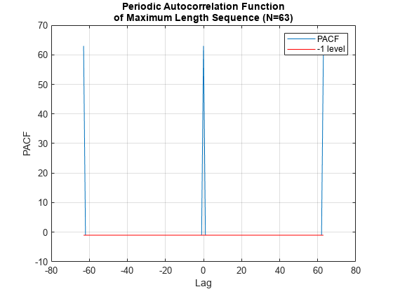
    Generate a length-63 maximum length sequence (MLS). Plot one period of the periodic autocorrelation function (PACF) to show that the PACF of an MLS has a constant sidelobe level of -1.

    N = 63;
    S = mlseq(N);

    Compute one period of the PACF.

    pacf = xcorr(S,[S;S;S],2*N);
    pacf = pacf(1:2*N+1);
    lag = -N:N;

    Plot the periodic autocorrelation function,

    plot(lag,pacf)
    grid on
    xlabel('Lag')
    ylabel('PACF')
    title({'Periodic Autocorrelation Function', ...
        sprintf('of Maximum Length Sequence (N=%d)',N)});
    hold on
    plot([-N N],[-1 -1],'r')
    legend('PACF','-1 level')
    hold off

    Figure contains an axes object. The axes object with title Periodic Autocorrelation Function of Maximum Length Sequence (N=63), xlabel Lag, ylabel PACF contains 2 objects of type line. These objects represent PACF, -1 level.

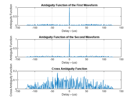
    Generate two phase-coded waveforms based on m-sequences of length N = 127. Show their ambiguity and crossambiguity functions. The chip width is 1μsec and the modulation period is N times the chip width.

    N = 127;
    S = mlseq(N,[1 2]);

    Set the chip width (tau) and the modulation period (T).

    tau = 1e-6; 
    T = tau*N;

    Create a custom phase coded waveform object. Set the pulse repetition frequency (PRF) equal to the inverse of the modulation period and set the sampling rate to 10 times the inverse chip width. Initialize the waveform with the first code.

    fs = 10/tau;    % Sample rate
    pmwaveform = phased.PhaseCodedWaveform('SampleRate',fs,'Code','Custom',...
        'CustomCode',S(:,1),'ChipWidth',tau,'PRF',1/T);

    Generate samples of the first waveform.

    x1 = pmwaveform();

    Generate samples of the second waveform.

    release(pmwaveform);
    pmwaveform.CustomCode = S(:,2);
    x2 = pmwaveform();

    Plot the ambiguity and cross-ambiguity functions.

    tiledlayout(3, 1)
    
    nexttile
    ambgfun(x1,fs,1/T,'Cut','Doppler');
    title('Ambiguity Function of the First Waveform')
    
    nexttile
    ambgfun(x2,fs,1/T,'Cut','Doppler');
    title('Ambiguity Function of the Second Waveform')
    
    nexttile
    ambgfun(x1,x2,fs,[1 1]/T,'Cut','Doppler');
    title('Cross Ambiguity Function')

    Figure contains 3 axes objects. Axes object 1 with title Ambiguity Function of the First Waveform, xlabel Delay {\tau} (us), ylabel Ambiguity Function contains an object of type line. Axes object 2 with title Ambiguity Function of the Second Waveform, xlabel Delay {\tau} (us), ylabel Ambiguity Function contains an object of type line. Axes object 3 with title Cross Ambiguity Function, xlabel Delay {\tau} (us), ylabel Cross Ambiguity Function contains an object of type line.

    Input Arguments

    collapse all

    Sequence length, specified as a positive integer. N must be an integer such that N=2n-1, where n is a positive integer. Allowable values for N are [7 15 31 63 127 255 511 1023 2047 4095 8191].

    Example: 1023

    Data Types: double

    Polynomial indices, specified as a positive integer or length-M vector of positive integers specifying the indices of primitive polynomials in GF(2n). Polynomial indices range from 1 to T where T is given in this table as a function of sequence length N or sequence index n.

    Polynomial indices

    N71531631272555112023204740958191
    n345678910111213
    T226618164860176144630

    Data Types: double

    Initial state of sequences, specified as a scalar or a length-M vector of positive integers from 1 to N. If both k and IS are specified as vectors they must have the same length.

    Output Arguments

    collapse all

    Maximum-length sequence, returned as a length-N column vector. The returned sequence is antipodal. Sequence elements can only take values of 1 and -1. If the input argument k is a scalar, the output S is a length-N column vector. If k is a length-M vector, the output S is an Nby-M matrix with columns corresponding to different sequences indexed by k.

    Primitive polynomial coefficients, returned as a real-valued length-n+1 column vector or real-valued (n+1)-by-M matrix. The rows of C correspond to the terms of the polynomials in the order of ascending power. If k is specified as a vector, the columns of C correspond to the different polynomials indexed by k.

    The function assigns an index of 1 to the polynomial whose coefficients C, when viewed as a sequence of bits (with the LSB corresponding to the power of 0), form the smallest integer. The index of T is assigned to the polynomial whose coefficients form the largest integer.

    • If the input k is a scalar, the output S is a column vector of length N.

    • If k is a length-M vector, the output argument S is an N-by-M matrix with columns corresponding to the different sequences indexed by k.

    Algorithms

    An MLS can be generated using a linear-feedback shift register. The taps of the register are set according to the non-zero coefficients of a primitive polynomial over Galois field GF(2n). A primitive polynomial in GF(2n) has a form

    m(x)=xn+cnxn1+cn1xn2+...+c1

    where ci is a length-n vector of coefficients. The entries of ci can either be 0 or 1 and can be interpreted as an integer in a binary form (MSB corresponds to the power of n-1). An MLS can then be generated using the recursion relation:

    si=mod(cnsi1cn1si2...c1sin,2)

    The first n elements of the sequence

    (s1,s2,...,sn)

    can be supplied as an initial condition in order to initiate the recursion. Choosing different initial conditions will result in different final sequences that are cyclic shifts of each other. There are total N=2n-1 possible initial conditions. The initial conditions can be represented as binary integers from 1 to N with the LSB corresponding to s1. The final step in generating the sequence to replacing the "0" entries with "-1". For a given n there can be multiple primitive polynomials in GF(2n) resulting in different sequences. By default, the function returns a sequence having the lowest autocorrelation sidelobes.

    References

    [1] Levanon, N. and E. Mozeson. Radar Signals. Hoboken, NJ: John Wiley & Sons, 2004.

    [2] Haderer, Heinz, Reinhard Feger, and Andreas Stelzer. "A comparison of phase-coded CW radar modulation schemes for integrated radar sensors" in 2014 44th European Microwave Conference, pp. 1896-1899. IEEE, 2014.

    Extended Capabilities

    C/C++ Code Generation
    Generate C and C++ code using MATLAB® Coder™.

    Version History

    Introduced in R2024a