Temperature Distribution in Heat Sink
This example shows how to create a simple 3-D heat sink geometry and analyze heat transfer on the heat sink.
Geometry
To create the geometry of a heat sink, first create a geometry of the base by using the multicylinder function.
gBase = multicuboid(0.01,0.008,0.0005);
gBase = translate(gBase,[0.005,0.004,0]);
gBase = fegeometry(gBase);
Plot the geometry.
pdegplot(gBase,CellLabels="on")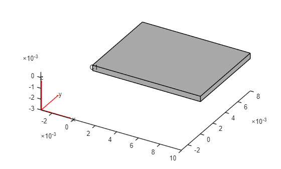
Create a geometry representing one fin.
gFin = multicylinder(0.0005,0.005);
gFin = fegeometry(gFin);
Now, create a geometry representing 12 fins by shifting the original fin to locations on top of the base.
g = fegeometry;
k = 0;
for i = 0.002:0.002:0.008
   for j = 0.002:0.002:0.006
       k = k + 1;
       gCylT(k) = translate(gFin,[i,j,0.0005]);
   end
end
Combine the geometry of the base with the geometries of the fins.
g = union(gBase,gCylT);
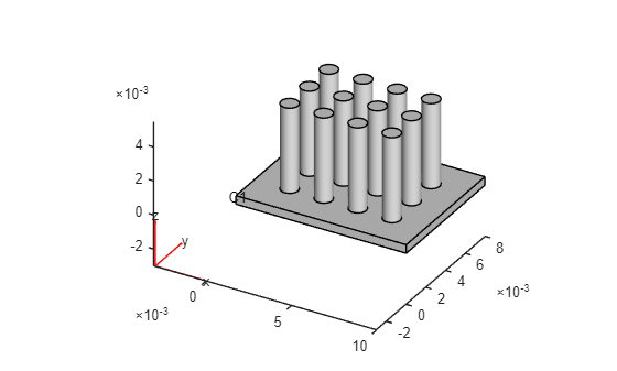
Plot the resulting heat sink geometry.
pdegplot(g,CellLabels="on")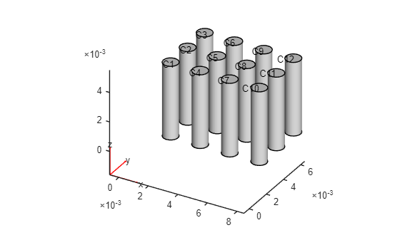
Thermal Analysis
Create an femodel object for transient thermal analysis and include the geometry.
model = femodel(AnalysisType="thermalTransient", ...
                Geometry = g);
Assuming that the heat sink is made of copper, specify the thermal conductivity, mass density, and specific heat.
model.MaterialProperties = ...
    materialProperties(ThermalConductivity=400, ...
                       MassDensity=8960, ...
                       SpecificHeat=386);
Specify the Stefan-Boltzmann constant.
model.StefanBoltzmann = 5.670367e-8;
Apply the temperature boundary condition on the bottom surface of the heat sink.
bottomFace = nearestFace(g,[0.0001,0.0001,0])
bottomFace =
25
model.FaceBC(bottomFace) = faceBC(Temperature=1000);
Specify the convection and radiation parameters on all other surfaces of the heat sink.
model.FaceLoad(setdiff(1:g.NumFaces,bottomFace)) = ...
    faceLoad(ConvectionCoefficient=5, ...
             AmbientTemperature=300, ...
             Emissivity=0.8);
Set the initial temperature of all the surfaces to the ambient temperature.
model.CellIC = cellIC(Temperature=300);
Generate a mesh.
model = generateMesh(model);
Solve the transient thermal problem for times between 0 and 0.0075 s with a time step of 0.0025 s.
results = solve(model,0:0.0025:0.0075);
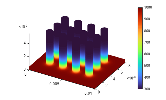
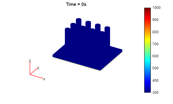
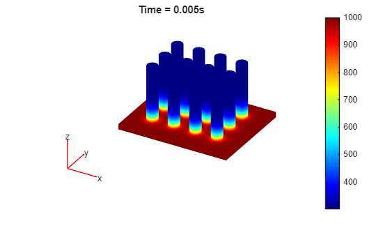
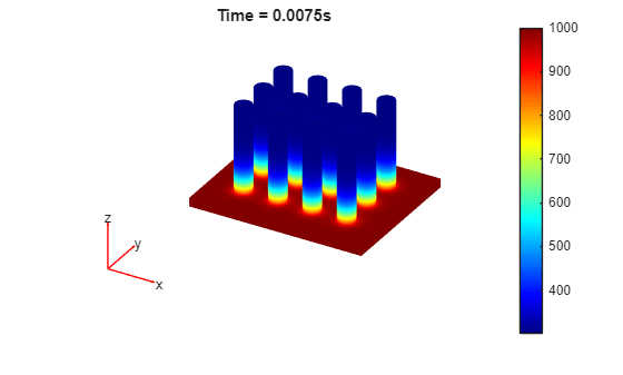
Plot the temperature distribution for each time step.
for i = 1:length(results.SolutionTimes)
  figure
  pdeplot3D(results.Mesh,ColorMapData=results.Temperature(:,i))
  title({['Time = ' num2str(results.SolutionTimes(i)) 's']})
end

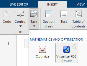
You also can plot the same results by using the Visualize PDE Results Live Editor task. First, create a new live script by clicking the New Live Script button in the File section on the Home tab.
On the Insert tab, select Task > Visualize PDE Results. This action inserts the task into your script.

To plot the temperature distribution for each time step, follow these steps.
In the Select results section of the task, select
resultsfrom the drop-down list.In the Specify data parameters section of the task, set Type to Temperature, and set the time steps to 1, 2, 3, and 4. These time steps correspond to the four time values that you used to solve the problem. You also can animate the solution by selecting Animate.