TransientThermalResults
Transient thermal solution and derived quantities
Description
A TransientThermalResults object contains
the temperature and gradient values in a form convenient for plotting and
postprocessing.
The temperature and its gradient are calculated at the nodes of the triangular or
tetrahedral mesh generated by generateMesh. Temperature values at the nodes
appear in the Temperature property. The solution times appear in the
SolutionTimes property. The three components of the temperature
gradient at the nodes appear in the XGradients,
YGradients, and ZGradients properties. You can
extract solution and gradient values for specified time indices from
Temperature, XGradients,
YGradients, and ZGradients.
To interpolate the temperature or its gradient to a custom grid (for example,
specified by meshgrid), use interpolateTemperature or evaluateTemperatureGradient.
To evaluate heat flux of a thermal solution at nodal or arbitrary spatial locations,
use evaluateHeatFlux. To evaluate integrated heat
flow rate normal to a specified boundary, use evaluateHeatRate.
Creation
Solve a transient thermal problem using the solve function. This function returns a transient thermal solution as a
TransientThermalResults object.
Properties
Object Functions
evaluateHeatFlux | Evaluate heat flux of thermal solution at nodal or arbitrary spatial locations |
evaluateHeatRate | Evaluate integrated heat flow rate normal to specified boundary |
evaluateTemperatureGradient | Evaluate temperature gradient of thermal solution at arbitrary spatial locations |
filterByIndex | Access transient results for specified time steps |
interpolateTemperature | Interpolate temperature in thermal result at arbitrary spatial locations |
Examples
Solve a 2-D transient thermal problem.
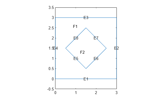
Create a geometry representing a square plate with a diamond-shaped region in its center.
SQ1 = [3; 4; 0; 3; 3; 0; 0; 0; 3; 3];
D1 = [2; 4; 0.5; 1.5; 2.5; 1.5; 1.5; 0.5; 1.5; 2.5];
gd = [SQ1 D1];
sf = 'SQ1+D1';
ns = char('SQ1','D1');
ns = ns';
g = decsg(gd,sf,ns);
pdegplot(g,EdgeLabels="on",FaceLabels="on")
xlim([-1.5 4.5])
ylim([-0.5 3.5])
axis equal
Create an femodel object for transient thermal analysis and include the geometry.
model = femodel(AnalysisType="thermalTransient", ...
                Geometry=g);
For the square region, assign these thermal properties:
Thermal conductivity is
Mass density is
Specific heat is
model.MaterialProperties(1) = ...
    materialProperties(ThermalConductivity=10, ...
                       MassDensity=2, ...
                       SpecificHeat=0.1);
For the diamond region, assign these thermal properties:
Thermal conductivity is
Mass density is
Specific heat is
model.MaterialProperties(2) = ...
    materialProperties(ThermalConductivity=2, ...
                       MassDensity=1, ...
                       SpecificHeat=0.1);
Assume that the diamond-shaped region is a heat source with a density of .
model.FaceLoad(2) = faceLoad(Heat=4);
Apply a constant temperature of 0 °C to the sides of the square plate.
model.EdgeBC(1:4) = edgeBC(Temperature=0);
Set the initial temperature to 0 °C.
model.FaceIC = faceIC(Temperature=0);
Generate the mesh.
model = generateMesh(model);
The dynamics for this problem are very fast. The temperature reaches a steady state in about 0.1 second. To capture the most active part of the dynamics, set the solution time to logspace(-2,-1,10). This command returns 10 logarithmically spaced solution times between 0.01 and 0.1.
tlist = logspace(-2,-1,10);
Solve the equation.
thermalresults = solve(model,tlist);
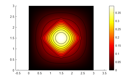
Plot the solution with isothermal lines by using a contour plot.
T = thermalresults.Temperature;
msh = thermalresults.Mesh;
pdeplot(msh,XYData=T(:,10),Contour="on",ColorMap="hot")
axis equal
Analyze heat transfer in a rod with a circular cross-section and internal heat generation by simplifying a 3-D axisymmetric model to a 2-D model.
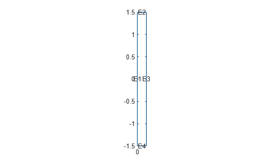
The 2-D model is a rectangular strip whose x-dimension extends from the axis of symmetry to the outer surface and whose y-dimension extends over the actual length of the rod (from -1.5 m to 1.5 m). Create the geometry by specifying the coordinates of its four corners. For axisymmetric analysis, the toolbox assumes that the axis of rotation is the vertical axis passing through r = 0.
g = decsg([3 4 0 0 .2 .2 -1.5 1.5 1.5 -1.5]');
Plot the geometry with the edge labels.
figure
pdegplot(g,EdgeLabels="on")
axis equal
Create an femodel for transient thermal analysis and include the geometry in the model.
model = femodel(AnalysisType="thermalTransient", ...
                Geometry=g);
Switch the type of the problem to axisymmetric.
model.PlanarType = "axisymmetric";The rod is composed of a material with these thermal properties.
k = 40; % thermal conductivity, W/(m*C)
rho = 7800; % density, kg/m^3
cp = 500; % specific heat, W*s/(kg*C)
q = 20000; % heat source, W/m^3
Specify the thermal conductivity, mass density, and specific heat of the material.
model.MaterialProperties = ...
    materialProperties(ThermalConductivity=k,...
                       MassDensity=rho,...
                       SpecificHeat=cp);
Specify internal heat source and boundary conditions.
model.FaceLoad = faceLoad(Heat=q);
Define the boundary conditions. There is no heat transferred in the direction normal to the axis of symmetry (edge 1). You do not need to change the default boundary condition for this edge. Edge 2 is kept at a constant temperature T = 100 °C.
model.EdgeBC(2) = edgeBC(Temperature=100);
Specify the convection boundary condition on the outer boundary (edge 3). The surrounding temperature at the outer boundary is 100 °C, and the heat transfer coefficient is .
model.EdgeLoad(3) = ...
    edgeLoad(ConvectionCoefficient=50, ...
             AmbientTemperature=100);
The heat flux at the bottom of the rod (edge 4) is .
model.EdgeLoad(4) = edgeLoad(Heat=5000);
Specify that the Initial temperature in the rod is zero.
model.FaceIC = faceIC(Temperature=0);
Generate the mesh.
model = generateMesh(model);
Compute the transient solution for solution times from t = 0 to t = 50000 seconds.
tfinal = 50000;
tlist = 0:100:tfinal;
result = solve(model,tlist);
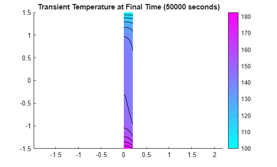
Plot the temperature distribution at t = 50000 seconds.
T = result.Temperature;

figure
pdeplot(result.Mesh,XYData=T(:,end), ...
                    Contour="on")
axis equal
title(sprintf(['Transient Temperature ' ...
               'at Final Time (%g seconds)'],tfinal))