Main Content

structuralBoundaryLoad

Specify boundary loads for structural model

Domain-specific structural workflow is not recommended. New features might not be compatible with this workflow. For help migrating your existing code to the unified finite element workflow, see Migration from Domain-Specific to Unified Workflow.

Description

structuralBoundaryLoad(structuralmodel,RegionType,RegionID,"SurfaceTraction",STval,"Pressure",Pval,"TranslationalStiffness",TSval) specifies the surface traction, pressure, and translational stiffness on the boundary of type RegionType with RegionID ID numbers.

  • Surface traction is determined as distributed normal and tangential forces acting on a boundary, resolved along the global Cartesian coordinate system.

  • Pressure must be specified in the direction that is normal to the boundary. A positive pressure value acts into the boundary (for example, compression). A negative pressure value acts away from the boundary (for example, suction).

  • Translational stiffness is a distributed spring stiffness for each translational direction. Translational stiffness is used to model an elastic foundation.

structuralBoundaryLoad does not require you to specify all three boundary loads. Depending on your structural analysis problem, you can specify one or more boundary loads by picking the corresponding arguments and omitting others. You can specify translational stiffness for any structural model. To specify pressure or surface traction, structuralmodel must be a static, transient, or frequency response model. Structural models for modal analysis cannot have pressure or surface traction.

The default boundary load is a stress-free boundary condition.

example

structuralBoundaryLoad(structuralmodel,"Vertex",VertexID,"Force",Fval) specifies concentrated force at a vertex with the VertexID number. You can specify force only if structuralmodel is a static, transient, or frequency response model. Structural models for modal analysis cannot have concentrated force.

example

structuralBoundaryLoad(___,"Vectorized","on") uses vectorized function evaluation when you pass a function handle as an argument. If your function handle computes in a vectorized fashion, then using this argument saves time. See Vectorization. For details on this evaluation, see Nonconstant Boundary Conditions.

Use this syntax with any of the input arguments from previous syntaxes.

structuralBoundaryLoad(___,"Pressure",Pval,Name,Value) lets you specify the form and duration of a nonconstant pressure pulse and harmonic excitation for a transient structural model without creating a function handle. When using this syntax, you must specify the model, region type and region ID, and pressure. Surface traction and translational stiffness are optional arguments. This syntax does not work for static, modal analysis, and frequency response models.

example

structuralBoundaryLoad(structuralmodel,"Vertex",VertexID,"Force",Fval,Name,Value) lets you specify the form and duration of a nonconstant concentrated force and harmonic excitation for a transient structural model without creating a function handle.

example

structuralBoundaryLoad(___,"Label",labeltext) adds a label for the structural boundary load to be used by the linearizeInput function. This function lets you pass boundary loads to the linearize function that extracts sparse linear models for use with Control System Toolbox™.

boundaryLoad = structuralBoundaryLoad(___) returns the boundary load object.

Examples

collapse all

Apply fixed boundaries and traction on two ends of a bimetallic cable.

Create a structural model.

structuralModel = createpde("structural","static-solid");

Create nested cylinders to model a bimetallic cable.

gm = multicylinder([0.01,0.015],0.05);

Assign the geometry to the structural model and plot the geometry.

structuralModel.Geometry = gm;
pdegplot(structuralModel,"CellLabels","on", ...
                         "FaceLabels","on", ...
                         "FaceAlpha",0.4)

Figure contains an axes object. The axes object contains 6 objects of type quiver, text, patch, line.

For each metal, specify Young's modulus and Poisson's ratio.

structuralProperties(structuralModel,"Cell",1,"YoungsModulus",110E9, ...
                                              "PoissonsRatio",0.28);
structuralProperties(structuralModel,"Cell",2,"YoungsModulus",210E9, ...
                                              "PoissonsRatio",0.3);

Specify that faces 1 and 4 are fixed boundaries.

structuralBC(structuralModel,"Face",[1,4],"Constraint","fixed")
ans = 
  StructuralBC with properties:

                RegionType: 'Face'
                  RegionID: [1 4]
                Vectorized: 'off'

   Boundary Constraints and Enforced Displacements
              Displacement: []
             XDisplacement: []
             YDisplacement: []
             ZDisplacement: []
                Constraint: "fixed"
                    Radius: []
                 Reference: []
                     Label: []

   Boundary Loads
                     Force: []
           SurfaceTraction: []
                  Pressure: []
    TranslationalStiffness: []
                     Label: []

Specify the surface traction for faces 2 and 5.

structuralBoundaryLoad(structuralModel, ...
                          "Face",[2,5], ...
                          "SurfaceTraction",[0;0;100])
ans = 
  StructuralBC with properties:

                RegionType: 'Face'
                  RegionID: [2 5]
                Vectorized: 'off'

   Boundary Constraints and Enforced Displacements
              Displacement: []
             XDisplacement: []
             YDisplacement: []
             ZDisplacement: []
                Constraint: []
                    Radius: []
                 Reference: []
                     Label: []

   Boundary Loads
                     Force: []
           SurfaceTraction: [3x1 double]
                  Pressure: []
    TranslationalStiffness: []
                     Label: []

Create a structural model.

structuralModel = createpde("structural","static-solid");

Create a block geometry.

gm = multicuboid(20,10,5);

Assign the geometry to the structural model and plot the geometry.

structuralModel.Geometry = gm;
pdegplot(structuralModel,"FaceLabels","on","FaceAlpha",0.5)

Figure contains an axes object. The axes object contains 6 objects of type quiver, text, patch, line.

Specify Young's modulus and Poisson's ratio.

structuralProperties(structuralModel,"YoungsModulus",30, ...
                                     "PoissonsRatio",0.3);

The bottom face of the block rests on an elastic foundation (a spring). To model this foundation, specify the translational stiffness.

structuralBoundaryLoad(structuralModel, ...
                              "Face",1, ...
                              "TranslationalStiffness",[0;0;30])
ans = 
  StructuralBC with properties:

                RegionType: 'Face'
                  RegionID: 1
                Vectorized: 'off'

   Boundary Constraints and Enforced Displacements
              Displacement: []
             XDisplacement: []
             YDisplacement: []
             ZDisplacement: []
                Constraint: []
                    Radius: []
                 Reference: []
                     Label: []

   Boundary Loads
                     Force: []
           SurfaceTraction: []
                  Pressure: []
    TranslationalStiffness: [3x1 double]
                     Label: []

Specify a force value at a vertex of a geometry.

Create a structural model for static analysis of a solid (3-D) problem.

model = createpde("structural","static-solid");

Create the geometry, which consists of two cuboids stacked on top of each other.

gm = multicuboid(0.2,0.01,[0.01 0.01],"Zoffset",[0 0.01]);

Include the geometry in the structural model.

model.Geometry = gm;

Plot the geometry and display the face labels. Rotate the geometry so that you can see the face labels on the left side.

figure 
pdegplot(model,"FaceLabels","on");
view([-67 5])

Figure contains an axes object. The axes object contains 6 objects of type quiver, text, patch, line.

Plot the geometry and display the vertex labels. Rotate the geometry so that you can see the vertex labels on the right side.

figure 
pdegplot(model,"VertexLabels","on","FaceAlpha",0.5)
xlim([-0.01 0.1])
zlim([-0.01 0.02])
view([60 5])

Figure contains an axes object. The axes object contains 6 objects of type quiver, text, patch, line.

Specify Young's modulus, Poisson's ratio, and the mass density of the material.

structuralProperties(model,"YoungsModulus",201E9,"PoissonsRatio",0.3);

Specify that faces 5 and 10 are fixed boundaries.

structuralBC(model,"Face",[5 10],"Constraint","fixed");

Specify the concentrated force at vertex 6.

structuralBoundaryLoad(model,"Vertex",6,"Force",[0;10^4;0])
ans = 
  StructuralBC with properties:

                RegionType: 'Vertex'
                  RegionID: 6
                Vectorized: 'off'

   Boundary Constraints and Enforced Displacements
              Displacement: []
             XDisplacement: []
             YDisplacement: []
             ZDisplacement: []
                Constraint: []
                    Radius: []
                 Reference: []
                     Label: []

   Boundary Loads
                     Force: [3x1 double]
           SurfaceTraction: []
                  Pressure: []
    TranslationalStiffness: []
                     Label: []

Use a function handle to specify a frequency-dependent pressure for a frequency response model.

Create a frequency response model for a 3-D problem.

fmodel = createpde("structural","frequency-solid");

Import and plot the geometry.

importGeometry(fmodel,"TuningFork.stl");
figure
pdegplot(fmodel,"FaceLabels","on")

Figure contains an axes object. The axes object contains 6 objects of type quiver, text, patch, line.

Specify the pressure loading on a tine (face 11) as a short rectangular pressure pulse. In the frequency domain, this pressure pulse is a unit load uniformly distributed across all frequencies.

structuralBoundaryLoad(fmodel,"Face",11,"Pressure",1);

Now specify a frequency-dependent pressure load, for example, p=e-(ω-1000)2/100000.

pLoad = @(location,state) exp(-(state.frequency-1E3).^2/1E5);
structuralBoundaryLoad(fmodel,"Face",12,"Pressure",pLoad);

Use a function handle to specify a harmonically varying pressure at the center of a thin 3-D plate.

Create a transient dynamic model for a 3-D problem.

structuralmodel = createpde("structural","transient-solid");

Create a geometry consisting of a thin 3-D plate with a small plate at the center. Include the geometry in the model and plot it.

gm = multicuboid([5,0.05],[5,0.05],0.01);
structuralmodel.Geometry = gm;
pdegplot(structuralmodel,"FaceLabels","on","FaceAlpha",0.5)

Figure contains an axes object. The axes object contains 6 objects of type quiver, text, patch, line.

Zoom in to see the face labels on the small plate at the center.

figure
pdegplot(structuralmodel,"FaceLabels","on","FaceAlpha",0.25)
axis([-0.2 0.2 -0.2 0.2 -0.1 0.1])

Figure contains an axes object. The axes object contains 6 objects of type quiver, text, patch, line.

Specify Young's modulus, Poisson's ratio, and the mass density of the material.

structuralProperties(structuralmodel,"YoungsModulus",210E9,...
                                     "PoissonsRatio",0.3,...
                                     "MassDensity",7800);

Specify that all faces on the periphery of the thin 3-D plate are fixed boundaries.

structuralBC(structuralmodel,"Constraint","fixed","Face",5:8);

Apply a harmonically varying pressure load on the small face at the center of the plate.

plungerLoad = @(location,state)5E7.*sin(25.*state.time);
structuralBoundaryLoad(structuralmodel,"Face",12,"Pressure",plungerLoad)
ans = 
  StructuralBC with properties:

                RegionType: 'Face'
                  RegionID: 12
                Vectorized: 'off'

   Boundary Constraints and Enforced Displacements
              Displacement: []
             XDisplacement: []
             YDisplacement: []
             ZDisplacement: []
                Constraint: []
                    Radius: []
                 Reference: []
                     Label: []

   Boundary Loads
                     Force: []
           SurfaceTraction: []
                  Pressure: @(location,state)5E7.*sin(25.*state.time)
    TranslationalStiffness: []
                     Label: []

   Time Variation of Force, Pressure, or Enforced Displacement
                 StartTime: []
                   EndTime: []
                  RiseTime: []
                  FallTime: []

   Sinusoidal Variation of Force, Pressure, or Enforced Displacement
                 Frequency: []
                     Phase: []

Specify a harmonically varying pressure at the center of a thin 3-D plate by specifying its frequency.

Create a transient dynamic model for a 3-D problem.

structuralmodel = createpde("structural","transient-solid");

Create a geometry consisting of a thin 3-D plate with a small plate at the center. Include the geometry in the model and plot it.

gm = multicuboid([5,0.05],[5,0.05],0.01);
structuralmodel.Geometry=gm;
pdegplot(structuralmodel,"FaceLabels","on","FaceAlpha",0.5)

Figure contains an axes object. The axes object contains 6 objects of type quiver, text, patch, line.

Zoom in to see the face labels on the small plate at the center.

figure
pdegplot(structuralmodel,"FaceLabels","on","FaceAlpha",0.25)
axis([-0.2 0.2 -0.2 0.2 -0.1 0.1])

Figure contains an axes object. The axes object contains 6 objects of type quiver, text, patch, line.

Specify Young's modulus, Poisson's ratio, and the mass density of the material.

structuralProperties(structuralmodel,"YoungsModulus",210E9,...
                                     "PoissonsRatio",0.3,...
                                     "MassDensity",7800);

Specify that all faces on the periphery of the thin 3-D plate are fixed boundaries.

structuralBC(structuralmodel,"Constraint","fixed","Face",5:8);

Apply a harmonically varying pressure load on the small face at the center of the plate.

structuralBoundaryLoad(structuralmodel,"Face",12, ...
                                       "Pressure",5E7, ...
                                       "Frequency",25)
ans = 
  StructuralBC with properties:

                RegionType: 'Face'
                  RegionID: 12
                Vectorized: 'off'

   Boundary Constraints and Enforced Displacements
              Displacement: []
             XDisplacement: []
             YDisplacement: []
             ZDisplacement: []
                Constraint: []
                    Radius: []
                 Reference: []
                     Label: []

   Boundary Loads
                     Force: []
           SurfaceTraction: []
                  Pressure: 50000000
    TranslationalStiffness: []
                     Label: []

   Time Variation of Force, Pressure, or Enforced Displacement
                 StartTime: []
                   EndTime: []
                  RiseTime: []
                  FallTime: []

   Sinusoidal Variation of Force, Pressure, or Enforced Displacement
                 Frequency: 25
                     Phase: []

Create a transient structural model.

structuralModel = createpde("structural","transient-solid");

Import and plot the geometry.

importGeometry(structuralModel,"BracketWithHole.stl");
pdegplot(structuralModel,"FaceLabels","on")
view(-20,10)

Figure contains an axes object. The axes object contains 6 objects of type quiver, text, patch, line.

Specify Young's modulus and Poisson's ratio.

structuralProperties(structuralModel,"YoungsModulus",200e9, ...
                                     "PoissonsRatio",0.3,...
                                     "MassDensity",7800);

Specify that face 4 is a fixed boundary.

structuralBC(structuralModel,"Face",4,"Constraint","fixed");

Apply a rectangular pressure pulse on face 7 in the direction normal to the face.

structuralBoundaryLoad(structuralModel,"Face",7,"Pressure",10^5,...
                                       "StartTime",0.1,"EndTime",0.5)
ans = 
  StructuralBC with properties:

                RegionType: 'Face'
                  RegionID: 7
                Vectorized: 'off'

   Boundary Constraints and Enforced Displacements
              Displacement: []
             XDisplacement: []
             YDisplacement: []
             ZDisplacement: []
                Constraint: []
                    Radius: []
                 Reference: []
                     Label: []

   Boundary Loads
                     Force: []
           SurfaceTraction: []
                  Pressure: 100000
    TranslationalStiffness: []
                     Label: []

   Time Variation of Force, Pressure, or Enforced Displacement
                 StartTime: 0.1000
                   EndTime: 0.5000
                  RiseTime: []
                  FallTime: []

   Sinusoidal Variation of Force, Pressure, or Enforced Displacement
                 Frequency: []
                     Phase: []

Specify a short concentrated force pulse at a vertex of a geometry.

Create a structural model for static analysis of a solid (3-D) problem.

structuralmodel = createpde("structural","transient-solid");

Create the geometry, which consists of two cuboids stacked on top of each other.

gm = multicuboid(0.2,0.01,[0.01 0.01],"Zoffset",[0 0.01]);

Include the geometry in the structural model.

structuralmodel.Geometry = gm;

Plot the geometry and display the face labels. Rotate the geometry so that you can see the face labels on the left side.

figure 
pdegplot(structuralmodel,"FaceLabels","on");
view([-67 5])

Figure contains an axes object. The axes object contains 6 objects of type quiver, text, patch, line.

Plot the geometry and display the vertex labels. Rotate the geometry so that you can see the vertex labels on the right side.

figure 
pdegplot(structuralmodel,"VertexLabels","on","FaceAlpha",0.5)
xlim([-0.01 0.1])
zlim([-0.01 0.02])
view([60 5])

Figure contains an axes object. The axes object contains 6 objects of type quiver, text, patch, line.

Specify Young's modulus, Poisson's ratio, and the mass density of the material.

structuralProperties(structuralmodel,"YoungsModulus",201E9, ...
                                     "PoissonsRatio",0.3, ...
                                     "MassDensity",7800);

Specify that faces 5 and 10 are fixed boundaries.

structuralBC(structuralmodel,"Face",[5 10],"Constraint","fixed");

Specify a short concentrated force pulse at vertex 6.

structuralBoundaryLoad(structuralmodel,"Vertex",6, ...
                                       "Force",[0;1000;0], ...
                                       "StartTime",1, ...
                                       "EndTime",1.05)
ans = 
  StructuralBC with properties:

                RegionType: 'Vertex'
                  RegionID: 6
                Vectorized: 'off'

   Boundary Constraints and Enforced Displacements
              Displacement: []
             XDisplacement: []
             YDisplacement: []
             ZDisplacement: []
                Constraint: []
                    Radius: []
                 Reference: []
                     Label: []

   Boundary Loads
                     Force: [3×1 double]
           SurfaceTraction: []
                  Pressure: []
    TranslationalStiffness: []
                     Label: []

   Time Variation of Force, Pressure, or Enforced Displacement
                 StartTime: 1
                   EndTime: 1.0500
                  RiseTime: []
                  FallTime: []

   Sinusoidal Variation of Force, Pressure, or Enforced Displacement
                 Frequency: []
                     Phase: []

Specify zero initial displacement and velocity.

structuralIC(structuralmodel,"Displacement",[0;0;0],"Velocity",[0;0;0]) 
ans = 
  GeometricStructuralICs with properties:

             RegionType: 'Cell'
               RegionID: [1 2]
    InitialDisplacement: [3×1 double]
        InitialVelocity: [3×1 double]

Generate a fine mesh.

generateMesh(structuralmodel,"Hmax",0.02);

Because the load is zero for the initial time span and is applied for only a short time, solve the model for two time spans. Use the first time span to find the solution before the force pulse.

structuralresults1 = solve(structuralmodel,0:1E-2:1); 

Use the second time span to find the solution during and after the force pulse.

structuralIC(structuralmodel,structuralresults1)
ans = 
  NodalStructuralICs with properties:

    InitialDisplacement: [1543×3 double]
        InitialVelocity: [1543×3 double]

structuralresults2 = solve(structuralmodel, ...
                     [1.001:0.001:1.01 1.02:1E-2:2]);

Plot the displacement value at the node corresponding to vertex 6, where you applied the concentrated force pulse.

loadedNd = findNodes(structuralmodel.Mesh,"region","Vertex",6); 
plot(structuralresults2.SolutionTimes, ...
     structuralresults2.Displacement.uy(loadedNd,:))

Figure contains an axes object. The axes object contains an object of type line.

Input Arguments

collapse all

Structural model, specified as a StructuralModel object. The model contains the geometry, mesh, structural properties of the material, body loads, boundary loads, and boundary conditions.

Example: structuralmodel = createpde("structural","transient-solid")

Geometric region type, specified as "Edge" for a 2-D model or "Face" for a 3-D model.

Example: structuralBoundaryLoad(structuralmodel,"Face",[2,5],"SurfaceTraction",[0,0,100])

Data Types: char | string

Geometric region ID, specified as a positive integer or vector of positive integers. Find the region IDs by using pdegplot.

Example: structuralBoundaryLoad(structuralmodel,"Face",[2,5],"SurfaceTraction",[0,0,100])

Data Types: double

Vertex ID, specified as a positive integer or vector of positive integers. Find the vertex IDs using pdegplot.

Example: structuralBoundaryLoad(structuralmodel,"Vertex",6,"Force",[0;10^4;0])

Data Types: double

Distributed normal and tangential forces on the boundary, resolved along the global Cartesian coordinate system, specified as a numeric vector or function handle. A numeric vector must contain two elements for a 2-D model and three elements for a 3-D model.

The function must return a two-row matrix for a 2-D model and a three-row matrix for a 3-D model. Each column of the matrix must correspond to the surface traction vector at the boundary coordinates provided by the solver. In case of a transient or frequency response analysis, STval also can be a function of time or frequency, respectively. For details, see More About.

Example: structuralBoundaryLoad(structuralmodel,"Face",[2,5],"SurfaceTraction",[0;0;100])

Data Types: double | function_handle

Pressure normal to the boundary, specified as a number or function handle. A positive-value pressure acts into the boundary (for example, compression), while a negative-value pressure acts away from the boundary (for example, suction).

If you specify Pval as a function handle, the function must return a row vector where each column corresponds to the value of pressure at the boundary coordinates provided by the solver. In case of a transient structural model, Pval also can be a function of time. In case of a frequency response structural model, Pval can be a function of frequency (when specified as a function handle) or a constant pressure with the same magnitude for a broad frequency spectrum. For details, see More About.

Example: structuralBoundaryLoad(structuralmodel,"Face",[2,5],"Pressure",10^5)

Data Types: double | function_handle

Distributed spring stiffness for each translational direction used to model elastic foundation, specified as a numeric vector or function handle. A numeric vector must contain two elements for a 2-D model and three elements for a 3-D model. The custom function must return a two-row matrix for a 2-D model and a three-row matrix for a 3-D model. Each column of this matrix corresponds to the stiffness vector at the boundary coordinates provided by the solver. In case of a transient or frequency response analysis, TSval also can be a function of time or frequency, respectively. For details, see More About.

Example: structuralBoundaryLoad(structuralmodel,"Edge",[2,5],"TranslationalStiffness",[0;5500])

Data Types: double | function_handle

Concentrated force at a vertex, specified as a numeric vector or function handle. Use a function handle to specify concentrated force that depends time or frequency. For details, see More About.

Example: structuralBoundaryLoad(structuralmodel,"Vertex",5,"Force",[0;0;10])

Data Types: double | function_handle

Label for the structural boundary load, specified as a character vector or a string.

Data Types: char | string

Name-Value Arguments

Example: structuralBoundaryLoad(structuralmodel,"Face",[2,5],"Pressure",10^5,"RiseTime",0.5,"FallTime",0.5,"EndTime",3)

Use one or more of the name-value pair arguments to specify the form and duration of the pressure or concentrated force pulse and harmonic excitation for a transient structural model only. Specify the pressure or force value using the Pval or Fval argument, respectively.

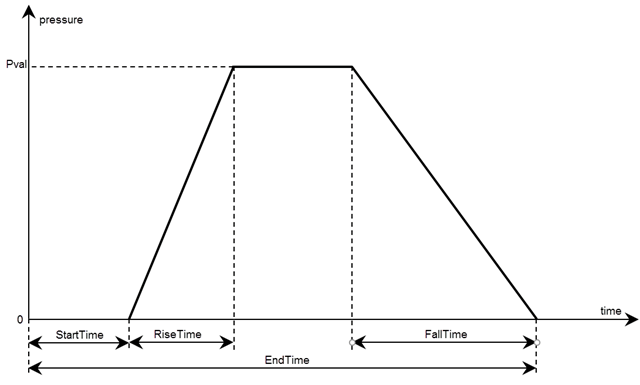
You can model rectangular, triangular, and trapezoidal pressure or concentrated force pulses. If the start time is 0, you can omit specifying it.

  • For a rectangular pulse, specify the start and end times.

  • For a triangular pulse, specify the start time and any two of the following times: rise time, fall time, and end time. You also can specify all three times, but they must be consistent.

  • For a trapezoidal pulse, specify all four times.

Trapezoidal pulse showing the start, rise, fall, and end times

You can model a harmonic pressure or concentrated force load by specifying its frequency and initial phase. If the initial phase is 0, you can omit specifying it.

Harmonic load showing the frequency and the initial phase

Rectangular, Triangular, or Trapezoidal Pulse

collapse all

Start time for pressure or concentrated force load, specified as a nonnegative number. Specify this argument only for transient structural models.

Example: structuralBoundaryLoad(structuralmodel,"Face",[2,5],"Pressure",10^5,"StartTime",1,"EndTime",3)

Data Types: double

End time for pressure or concentrated force load, specified as a nonnegative number equal or greater than the start time value. Specify this argument only for transient structural models.

Example: structuralBoundaryLoad(structuralmodel,"Face",[2,5],"Pressure",10^5,"StartTime",1,"EndTime",3)

Data Types: double

Rise time for pressure or concentrated force load, specified as a nonnegative number. Specify this argument only for transient structural models.

Example: structuralBoundaryLoad(structuralmodel,"Face",[2,5],"Pressure",10^5,"RiseTime",0.5,"FallTime",0.5,"EndTime",3)

Data Types: double

Fall time for pressure or concentrated force load, specified as a nonnegative number. Specify this argument only for transient structural models.

Example: structuralBoundaryLoad(structuralmodel,"Face",[2,5],"Pressure",10^5,"RiseTime",0.5,"FallTime",0.5,"EndTime",3)

Data Types: double

Harmonic Pressure or Force

collapse all

Frequency of sinusoidal pressure or concentrated force, specified as a positive number, in radians per unit of time. Specify this argument only for transient structural models.

Example: structuralBoundaryLoad(structuralmodel,"Face",[2,5],"Pressure",10^5,"Frequency",25)

Data Types: double

Phase of sinusoidal pressure or concentrated force, specified as a nonnegative number, in radians. Specify this argument only for transient structural models.

Example: structuralBoundaryLoad(structuralmodel,"Face",[2,5],"Pressure",10^5,"Frequency",25,"Phase",pi/6)

Data Types: double

Output Arguments

collapse all

Handle to boundary load, returned as a StructuralBC object. See StructuralBC Properties.

More About

collapse all

Specifying Nonconstant Parameters of a Structural Model

Use a function handle to specify the following structural parameters when they depend on space and, depending of the type of structural analysis, either time or frequency:

  • Surface traction on the boundary

  • Pressure normal to the boundary

  • Concentrated force at a vertex

  • Distributed spring stiffness for each translational direction used to model elastic foundation

  • Enforced displacement and its components

  • Initial displacement and velocity (can depend on space only)

For example, use function handles to specify the pressure load, x-component of the enforced displacement, and the initial displacement for this model.

structuralBoundaryLoad(model,"Face",12, ...
                             "Pressure",@myfunPressure)
structuralBC(model,"Face",2, ...
                   "XDisplacement",@myfunBC)
structuralIC(model,"Face",12, ...
                   "Displacement",@myfunIC)

For all parameters, except the initial displacement and velocity, the function must be of the form:

function structuralVal = myfun(location,state)

For the initial displacement and velocity the function must be of the form:

function structuralVal = myfun(location)

The solver computes and populates the data in the location and state structure arrays and passes this data to your function. You can define your function so that its output depends on this data. You can use any names instead of location and state, but the function must have exactly two arguments (or one argument if the function specifies the initial displacement or initial velocity).

  • location — A structure containing these fields:

    • location.x — The x-coordinate of the point or points

    • location.y — The y-coordinate of the point or points

    • location.z — For a 3-D or an axisymmetric geometry, the z-coordinate of the point or points

    • location.r — For an axisymmetric geometry, the r-coordinate of the point or points

    Furthermore, for boundary conditions, the solver passes these data in the location structure:

    • location.nxx-component of the normal vector at the evaluation point or points

    • location.nyy-component of the normal vector at the evaluation point or points

    • location.nz — For a 3-D or an axisymmetric geometry, z-component of the normal vector at the evaluation point or points

    • location.nr — For an axisymmetric geometry, r-component of the normal vector at the evaluation point or points

  • state — A structure containing these fields for dynamic structural problems:

    • state.time contains the time at evaluation points.

    • state.frequency contains the frequency at evaluation points.

    state.time and state.frequency are scalars.

Boundary constraints and loads get these data from the solver:

  • location.x, location.y, location.z, location.r

  • location.nx, location.ny, location.nz, location.nr

  • state.time or state.frequency (depending of the type of structural analysis)

Initial conditions get these data from the solver:

  • location.x, location.y, location.z, location.r

  • Subdomain ID

If a parameter represents a vector value, such as surface traction, spring stiffness, force, or displacement, your function must return a two-row matrix for a 2-D model and a three-row matrix for a 3-D model. Each column of the matrix corresponds to the parameter value (a vector) at the boundary coordinates provided by the solver.

If a parameter represents a scalar value, such as pressure or a displacement component, your function must return a row vector where each element corresponds to the parameter value (a scalar) at the boundary coordinates provided by the solver.

If boundary conditions depend on state.time or state.frequency, ensure that your function returns a matrix of NaN of the correct size when state.frequency or state.time are NaN. Solvers check whether a problem is nonlinear or time dependent by passing NaN state values and looking for returned NaN values.

Additional Arguments in Functions for Nonconstant Structural Parameters

To use additional arguments in your function, wrap your function (that takes additional arguments) with an anonymous function that takes only the location and state arguments. For example:

structuralVal = ...
@(location,state) myfunWithAdditionalArgs(location,state,arg1,arg2...)
structuralBC(model,"Face",2,"XDisplacement",structuralVal)

structuralVal = ...
@(location) myfunWithAdditionalArgs(location,arg1,arg2...)
structuralIC(model,"Face",2,"Displacement",structuralVal)

Version History

Introduced in R2017b

expand all