3-D Battery Module Cooling Analysis Using Fourier Neural Operator

Since R2026a

This example shows how to model three-dimensional heat diffusion in a battery module using a Fourier neural operator (FNO) neural network.

A neural operator [1] is a type of neural network that maps between function spaces. For example, it can learn to output the solution to a partial differential equation (PDE) when given the initial conditions of the system. A Fourier neural operator (FNO) [2] is a neural operator that can learn these mappings more efficiently by leveraging Fourier transforms. The FNO operates in the frequency domain and enables efficient learning of global patterns. Using a neural network to predict the PDE solutions can be significantly faster than computing the solutions numerically.

You can use FNO neural networks for tasks that involve learning mappings between input parameters and PDE solutions, such as fluid dynamics, heat transfer, and structural mechanics.

For demonstration purposes, this example trains the model using synthetically generated data. If you have your own simulation or experimental data, you can adapt the example accordingly to use your own data. The example creates the geometry of the battery module and solves the heat equation using functionality from Partial Differential Equation Toolbox™. You can vary some of the material and physical properties that define the PDE to create a collection of experiments. The task is to learn the mapping from a set of material and physical properties to the temperature at a future time.

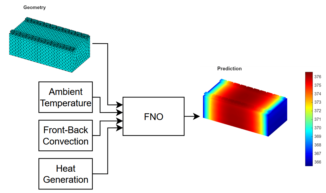
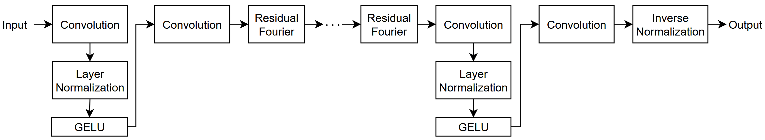
This diagram shows the flow of data through the FNO neural network trained in this example.

For an example that shows how to use a built-in reduced-order model (ROM) for this task that solves the underlying PDE accurately and quickly, see Battery Module Cooling Analysis and Reduced-Order Thermal Model. Similar to an FNO neural network, built-in ROMs can provide fast approximations of PDE solutions. Advantages of using an FNO neural network over built-in ROMs include:

• Data-driven modeling: The FNO model does not require knowledge or information about the underlying physical system and you can apply it to different types of PDE tasks.

• Flexible prediction: Using an FNO, you can quickly approximate solutions for many different input parameters.

• Zero-shot super-resolution (ZSSR): Because an FNO neural network learns mappings between function spaces, you can evaluate the output function at a higher resolution than that of the training data. That is, the network can enhance the resolution of the input and output data beyond the original training data.

The data generation and training steps in this example take a long time to run. By default, this example skips the data generation and network training and instead downloads the generated data and a trained network. To perform data generation and training, set the doGeneration and doTraining variables to true, respectively.

doGeneration = false;
doTraining = false;

Create Battery Module Geometry

Specify the sizes for the battery module geometry. Specify the number of cells in the module and the sizes of the cells, tabs, and connectors.

numCellsInModule = 20;

cellWidth = 0.150;
cellThickness = 0.015;
tabThickness = 0.01;
tabWidth = 0.015;
cellHeight = 0.1;
tabHeight = 0.005;
connectorHeight = 0.003;

Create the battery module geometry using the createBatteryModuleGeometry function, attached to this example as a supporting file. To access this function, open this example as a live script.

[geomModule, volumeIDs, boundaryIDs, volume] = createBatteryModuleGeometry( ...
    numCellsInModule,cellWidth,cellThickness,tabThickness, ...
    tabWidth,cellHeight,tabHeight,connectorHeight);

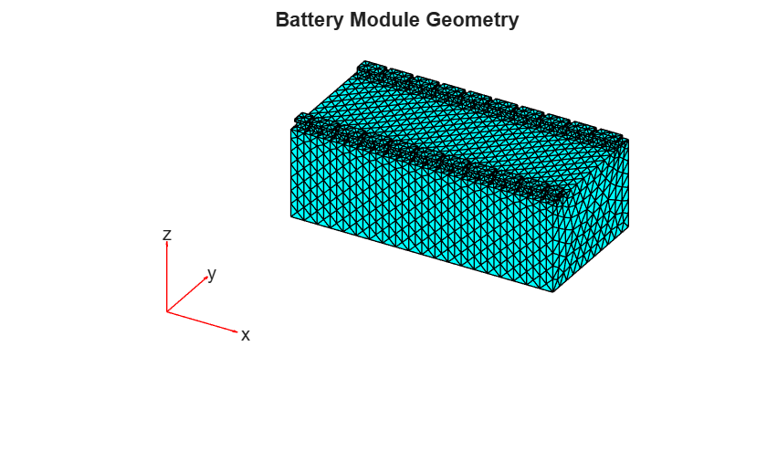
Create a finite element analysis model object from the geometry and visualize it in a PDE mesh plot.

model = femodel( ...
    AnalysisType="thermalTransient", ...
    Geometry=geomModule);

model = generateMesh(model);
pdemesh(model)
title("Battery Module Geometry")

Generate Training Data

Generate a data set of temperature distributions by solving the heat equation for different combinations of physical and environmental parameters.

Specify the thermal conductivity of the battery in watts per meter-kelvin (W/(K*m)).

throughPlaneConductivity = 2;
inPlaneConductivity = 80;
thermalConductivityTab = 386;
thermalConductivityConnector = 400;

Specify the mass densities of the battery components in kilograms per cubic meter (kg/m³).

densityCell = 780;
densityTab = 2700;
densityConnector = 540;

Specify the specific heat values of the battery components in joules per kilogram-kelvin (J/(kg*K)).

heatCell = 785;
heatTab = 890;
heatConnector = 840;

To generate parameters for a range of simulation inputs, specify the minimum and maximum values of the ambient temperature, convection coefficients, and heat generation rates. For each range, specify to use 6 regularly spaced values.

numValues = 6;

minAmbientTemperature = 280;
maxAmbientTemperature = 300;

minFrontBackConvection = 10;
maxFrontBackConvection = 20;

minHeatGeneration = 10;
maxHeatGeneration = 20;

Specify the number of time steps to solve the model for. This example uses a value of $$T=600$$ (10 minutes).

T = 600;

Create arrays containing a range of values for the ambient temperature, convection coefficients, and heat generation rates.

ambientTemperature = linspace(minAmbientTemperature,maxAmbientTemperature,numValues);
frontBackConvection = linspace(minFrontBackConvection,maxFrontBackConvection,numValues);
heatGeneration = linspace(minHeatGeneration,maxHeatGeneration,numValues);

Combine the through-plane and in-plane conductivity values.

thermalConductivityCell = [ ...
    throughPlaneConductivity
    inPlaneConductivity
    inPlaneConductivity];

Collect IDs for assigning material properties and boundary conditions.

cellIDs = [volumeIDs.Cell];
tabIDs = [volumeIDs.TabLeft volumeIDs.TabRight];
connectorIDs = [volumeIDs.ConnectorLeft volumeIDs.ConnectorRight];

Assign the material properties of the cell body, tabs, and connectors.

model.MaterialProperties(cellIDs) = materialProperties( ...
    ThermalConductivity=thermalConductivityCell, ...
    MassDensity=densityCell, ...
    SpecificHeat=heatCell);

model.MaterialProperties(tabIDs) = materialProperties( ...
    ThermalConductivity=thermalConductivityTab, ...
    MassDensity=densityTab, ...
    SpecificHeat=heatTab);

model.MaterialProperties(connectorIDs) = materialProperties( ...
    ThermalConductivity=thermalConductivityConnector, ...
    MassDensity=densityConnector, ...
    SpecificHeat=heatConnector);

Create an array of all combinations of varying parameters using the combinations function.

tbl = combinations(ambientTemperature,frontBackConvection,heatGeneration);
parameters = tbl.Variables;

To generate the data, solve the transient heat equation by looping through each parameter combination. For each combination, assign the corresponding boundary and source conditions, then solve the model using solve function of the femodel object. To later compare the time it takes to compute the solutions numerically versus using the neural network trained in this example, time the data generation process.

This step can take a long time to run. The example downloads the results. To generate the data, set the doGeneration variable to true.

if doGeneration
    tic
    fprintf("Generating data... ")

    results = cell(size(parameters,1),1);

    faceIDs = [boundaryIDs(1).FrontFace boundaryIDs(end).BackFace];

    for i = 1:size(parameters,1)
        model.FaceLoad(faceIDs) = faceLoad( ...
            ConvectionCoefficient=parameters(i,2), ...
            AmbientTemperature=parameters(i,1));

        nominalHeat = parameters(i,3)/volume(1).Cell;
        model.CellLoad(cellIDs) = cellLoad(Heat=nominalHeat);

        model.CellIC = cellIC(Temperature=parameters(i,1));

        results{i} = solve(model,[0 T]);
    end
    elapsedGeneration = toc;
    fprintf("Done.\n")
    fprintf("Data generation time: %f seconds.\n",elapsedGeneration)
else
    fprintf("Downloading data... ")
    filenameData = matlab.internal.examples.downloadSupportFile("nnet","data/BatteryModuleCoolingData.mat");
    load(filenameData)
    fprintf("Done.\n")
end

Downloading data... 

Done.

Visualize one of the observations.

i = 1;
result = results{i};
target = result.Temperature(:,end);

tempMin = min(target);
tempMax = max(target);

figure
pdeplot3D(result.Mesh, ...
    ColorMapData=target, ...
    FaceAlpha=1);

clim([tempMin tempMax]);
title("Training Observation")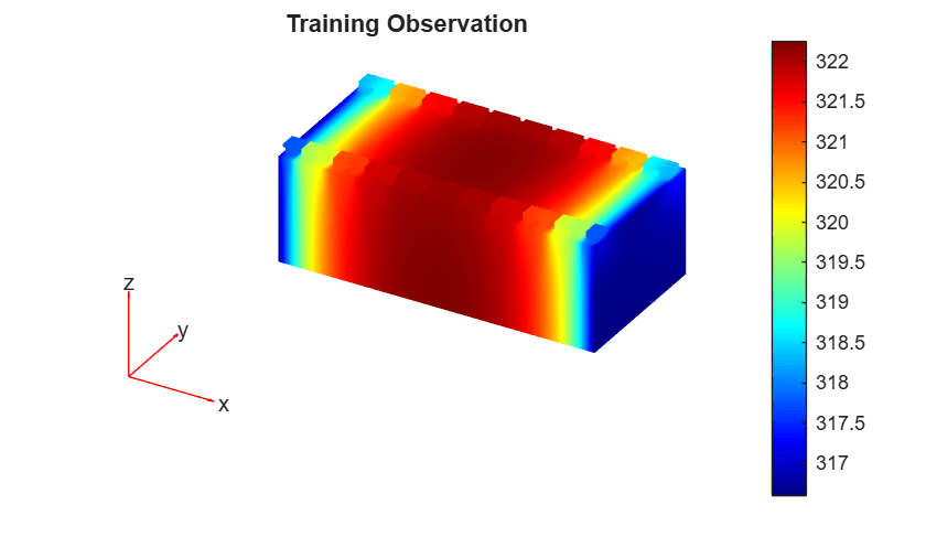

Prepare Data for Training

Fourier neural operators require the data to be aligned on a regular grid of points, like those that meshgrid and ndgrid create.

At each point $$(x_i,y_i,z_i)$$ on the grid these physical properties vary:

• The ambient temperature $$T_i$$,

• The convection $$P_i$$

• The heat generation $$Q_i$$

These varying physical properties are the input features $$u$$. The targets $$v$$ are the corresponding temperatures of the points at the end of the simulation.

By considering $$T_i$$, $$P_i$$, and $$Q_i$$ as functions of the points $$(x_i,y_i,z_i)$$ and extending these functions to take a value of zero at the unspecified vertices, you can consider the function $$u_i(x,y,z)=(x,y,z,T_i(x,y,z),P_i(x,y,z),Q_i(x,y,z))$$ as a representation of the input data.

The results from the data generation step are the values of $$u_i$$ and $$v_i$$ aligned to the mesh vertices. You can interpolate these aligned points onto a regular grid. This gives a 5-dimensional array U. The dimensions of the array correspond to different details of the data:

• The first three dimensions index into the spatial coordinates.

• The fourth dimension indexes into the input features.

• The fifth dimension indexes into the observations.

Specify a grid size of 32.

gridSize = 32;

Get the bounds of the mesh.

XYZ = geomModule.Mesh.Nodes;

xMin = min(XYZ(1,:));
xMax = max(XYZ(1,:));

yMin = min(XYZ(2,:));
yMax = max(XYZ(2,:));

zMin = min(XYZ(3,:));
zMax = max(XYZ(3,:));

Create the grid coordinates.

x = linspace(xMin,xMax,gridSize);
y = linspace(yMin,yMax,gridSize);
z = linspace(zMin,zMax,gridSize);

[X,Y,Z] = meshgrid(x,y,z);

Interpolate temperature, convection, and heat generation onto a regular grid. Impute missing values, then assemble input-output tensors for training. For each parameter:

• Calculate the targets by interpolating the final temperature onto the regular grid using the interpolateTemperature function. Find any NaN values and impute them by projecting up from the last non-NaN value in the $$z$$-dimension. NaN values occur when grid coordinates lie outside the geometry. For example, NaN values can occur when the tabs on the battery module extend in the $$z$$-dimension.

• Create functions for the convection aligned onto the nodes.

• Interpolate the convection and heat generation data to the grid points using the scatteredInterpolant function.

• Specify the ambient temperature as a constant feature, and append the convection and heat generation interpolated features.

• Add the data to the U and V variables.

Use the findNodes function to get the node indices where material properties are specified, and interpolate a function that has the specified property value at those nodes, and zero elsewhere. This approach of extending values as zero makes physical sense because in the PDE formulation, boundary conditions and source terms are naturally represented this way. When a physical property (like convection) only applies at specific boundaries or regions, it has no effect elsewhere in the domain, which corresponds to a value of zero. Similarly, heat generation only occurs within the battery cells and is zero elsewhere. By representing the data this way, this maintains the physical meaning of these parameters while creating a consistent format for the neural network to learn from.

This step can take a long time to run. The example downloads the results. To interpolate the generated data, set the doGeneration variable to true.

F = scatteredInterpolant(model.Mesh.Nodes.', zeros(size(model.Mesh.Nodes,2),1));

if doGeneration
    tic
    fprintf("Generating data... ")

    numParameters = size(parameters,1);
    U = zeros(gridSize,gridSize,gridSize,numValues,numParameters);
    V = zeros(gridSize,gridSize,gridSize,1,numParameters);

    for i = 1:numParameters
        result = results{i};

        % Interpolate the final temperature onto the regular grid.
        idxT = length(result.SolutionTimes);
        T = interpolateTemperature(result,X(:),Y(:),Z(:),idxT);
        T = reshape(T,gridSize,gridSize,gridSize);

        % Find NaN values and impute along the z-dimension.
        T = fillmissing(T,"previous",3);

        % Specify functions for the convection aligned
        % onto the face load nodes.
        boundary = findNodes(result.Mesh,"region",Face=faceIDs);
        convection = zeros(size(result.Mesh.Nodes,2),1);
        convection(boundary) = parameters(i,2);

        % Interpolate the convection to the grid points.
        F.Values = convection;
        convectionGrid = F(X,Y,Z);

        % Interpolate the heat generation.
        cells = findNodes(result.Mesh,"region",Cell=cellIDs);
        heatGeneration = zeros(size(result.Mesh.Nodes,2),1);
        heatGeneration(cells) = parameters(i,3);

        F.Values = heatGeneration; 
        heatGenerationGrid = F(X,Y,Z);

        % Specify the ambient temperature as a constant feature, and append the
        % convection and heat generation interpolated features.
        ambientTemperature = repmat(parameters(i,1),size(convectionGrid));

        U(:,:,:,1:3,i) = cat(4,X,Y,Z);
        U(:,:,:,4:end,i) = cat(4,ambientTemperature,convectionGrid,heatGenerationGrid);
        V(:,:,:,:,i) = T;
    end
    
    fprintf("Done.\n")
    toc
else
    fprintf("Downloading data... ")
    filenameDataInterpolated = matlab.internal.examples.downloadSupportFile("nnet","data/BatteryModuleCoolingDataInterpolated.mat");
    load(filenameDataInterpolated)
    fprintf("Done.\n")
end

Downloading data... 

Done.

Split the data into training, validation, and test partitions using the trainingPartitions function, which is attached to this example as a supporting file. To access this function, open the example as a live script. Use 80% of the data for training and the remaining 20% for validation.

numObservations = size(U,5);
[idxTrain,idxValidation] = trainingPartitions(numObservations,[0.8 0.2]);

UTrain = U(:,:,:,:,idxTrain);
UValidation = U(:,:,:,:,idxValidation);

VTrain = V(:,:,:,:,idxTrain);
VValidation = V(:,:,:,:,idxValidation);

Define 3-D Fourier Layer

Create a function that returns a networkLayer object that represents a 3-D Fourier layer with residual connections.

function layer = residualFourier3dLayer(numModes,hiddenSize)

net = dlnetwork;

layers = [
    identityLayer(Name="in")
    spectralConvolution3dLayer(numModes,hiddenSize)
    additionLayer(2,Name="add")
    layerNormalizationLayer
    geluLayer
    additionLayer(2,Name="add2")];

net = addLayers(net,layers);

layer = convolution3dLayer(1,hiddenSize,Name="conv");
net = addLayers(net,layer);

net = connectLayers(net,"in","conv");
net = connectLayers(net,"conv","add/in2");
net = connectLayers(net,"in","add2/in2");

layer = networkLayer(net);

end

Define Neural Network Architecture

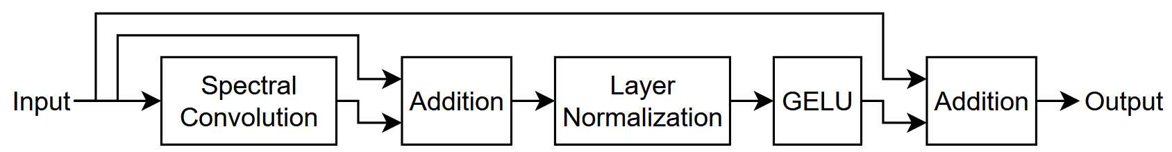
This diagram illustrates the FNO neural network architecture.

Create a layer array that specifies the neural network architecture.

• To input the data as a 3-D volume, use an image input layer. The size of the spatial dimensions match the grid size, the size of the channel dimension matches the number of channels of the input data.

• For the learnable layers, specify a base hidden size of 64.

• Use four residual Fourier layers and set the number of modes and the hidden size four and the base hidden size.

• For the first and third convolution layers, set the convolutional filter size and number of convolutional filters to one and twice the base hidden size, respectively.

• For the second convolution layer, set the convolutional filter size and number of convolutional filters to one and base hidden size, respectively.

• For the final convolution layer, use one filter with a size that matches the number of channels of the targets.

• For the convolution layers, pad the layer input data so that the output data has the same size.

• Finally, to apply the inverse target normalization operation when making predictions with the network, include an inverse normalization layer. During training, this layer has no effect.

numResidualLayers = 4;
hiddenSize = 64;
numModes = 4;

layers = [
    image3dInputLayer([gridSize,gridSize,gridSize,size(U,4)])
    convolution3dLayer(1,2*hiddenSize,Padding="same")
    layerNormalizationLayer
    geluLayer
    convolution3dLayer(1,hiddenSize,Padding="same")
    repmat(residualFourier3dLayer(numModes,hiddenSize),numResidualLayers,1)
    convolution3dLayer(1,2*hiddenSize,Padding="same")  
    layerNormalizationLayer
    geluLayer
    convolution3dLayer(1,size(V,4),Padding="same")
    inverseNormalizationLayer];

Specify Training Options

Specify the training options. Choosing among the options requires empirical analysis. To explore different training option configurations by running experiments, you can use the Experiment Manager (Deep Learning Toolbox) app.

• Train using the Adam solver for 1000 epochs with a mini-batch size of 8.

• Normalize the target data.

• Shuffle the data every epoch.

• Validate the neural network using the validation data every 100 iterations.

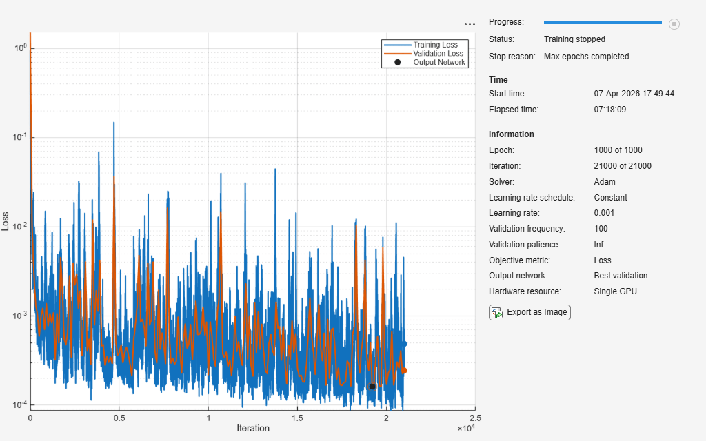
• Monitor the training progress in a plot and disable the verbose output.

options = trainingOptions("adam", ...
    NormalizeTargets=true, ...
    MaxEpochs=1000, ...
    MiniBatchSize=8, ...
    Shuffle="every-epoch", ...
    ValidationData={UValidation,VValidation}, ...
    ValidationFrequency=100, ...
    Plots="training-progress", ...
    Verbose=false);

Train Neural Network

Train the neural network using the trainnet (Deep Learning Toolbox) function. For regression, use $$L_2$$ loss. By default, the trainnet function uses a GPU if one is available. Using a GPU requires a Parallel Computing Toolbox™ license and a supported GPU device. For information on supported devices, see GPU Computing Requirements (Parallel Computing Toolbox). Otherwise, the function uses the CPU. To select the execution environment manually, use the ExecutionEnvironment training option.

This step can take a long time to run. Using an NVIDIA Titan RTX with 24 GB of memory, the neural network takes about 6 hours to train. The example downloads the trained network. To train the network, set the doTraining variable to true.

To inspect the loss more closely, set the y-axis to a log scale using the plot controls.

if doTraining
    [net,info] = trainnet(UTrain,VTrain,layers,"l2loss",options);
else
    fprintf("Downloading network... ")
    filenameNetwork = matlab.internal.examples.downloadSupportFile("nnet","data/BatteryModuleCoolingNetwork.mat");
    load(filenameNetwork)
    show(info)
    fprintf("Done.\n")
end

Downloading network... 

Done.

Test Neural Network

Test the neural network using the testnet function. Calculate the root mean squared error (RMSE) using the validation data. A lower value indicates a better fit for the validation data.

rmseValidation = testnet(net,UValidation,VValidation,"rmse")

rmseValidation = 
0.2199

Investigate the network predictions. Make predictions using the minibatchpredict (Deep Learning Toolbox) function. By default, the minibatchpredict function uses a GPU if one is available. Otherwise, the function uses the CPU. To select the execution environment manually, use the ExecutionEnvironment option.

tic
VPredictionsValidation = minibatchpredict(net,UValidation);
elapsedPrediction = toc

elapsedPrediction = 
2.7703

To compare the prediction time with time it takes to compute the solutions numerically, compare the average per-observation prediction time with the average per-observation elapsed time of generating the targets for training.

To compute the per-observation elapsed time, divide the elapsed time values for the data generation process and the predictions by the total number of observations and the number of validation observations, respectively.

timePerObservationGeneration = elapsedGeneration/size(U,5);
timePerObservationModel = elapsedPrediction/size(UValidation,5);

Visualize the times in a bar chart. In this example, making predictions with the FNO neural network is significantly faster.

figure
bar(["Numeric Solutions" "FNO Solutions"],[timePerObservationGeneration timePerObservationModel]);
ylabel("Time (s)")
title("Computation Time Per Observation")

Visualize one of the predictions in a plot. Select one of the predictions at random.

i = randi([1 size(UValidation,2)]);

To compare the predictions to the corresponding numerically computed solution, interpolate the predictions so that the points lie on the original mesh. To interpolate the predictions, use a griddedInterpolant object. Because the griddedInterpolant object requires the data to be in ndgrid format, permute the data.

P = [2 1 3];
result = results{idxValidation(i)};

interpolation = griddedInterpolant( ...
    permute(X,P), ...
    permute(Y,P), ...
    permute(Z,P), ...
    permute(VPredictionsValidation(:,:,:,:,i),P), ...
    "spline");

prediction = interpolation(result.Mesh.Nodes.');

Calculate the difference between the interpolated predictions and the numerically computed solutions.

target = result.Temperature(:,end);
diffMesh = abs(prediction - target);

Calculate the limits for the PDE plot.

tempMin = min([target; prediction]);
tempMax = max([target; prediction]);

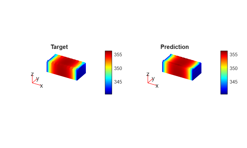
Visualize the prediction in a 3-D PDE plot.

figure
tiledlayout(1,2);

nexttile(1);
pdeplot3D(result.Mesh, ...
    ColorMapData=target, ...
    FaceAlpha=1);

clim([tempMin tempMax]);

title("Target")

nexttile(2);
pdeplot3D(result.Mesh, ...
    ColorMapData=prediction, ...
    FaceAlpha=1);

clim([tempMin tempMax]);

title("Prediction")

Visualize the absolute error in a 3-D PDE plot.

figure
pdeplot3D(result.Mesh, ...
    ColorMapData=diffMesh, ...
    FaceAlpha=1);

title("Absolute Error")

References

1. Li, Zongyi, Nikola Kovachki, Kamyar Azizzadenesheli, Burigede Liu, Kaushik Bhattacharya, Andrew Stuart, and Anima Anandkumar. "Neural Operator: Graph Kernel Network for Partial Differential Equations." arXiv, March 6, 2020. http://arxiv.org/abs/2003.03485.

2. Li, Zongyi, Nikola Kovachki, Kamyar Azizzadenesheli, Burigede Liu, Kaushik Bhattacharya, Andrew Stuart, and Anima Anandkumar. “Fourier Neural Operator for Parametric Partial Differential Equations,” 2020. https://openreview.net/forum?id=c8P9NQVtmnO.