Check lsqcurvefit Gradient

When you provide gradient evaluation functions, nonlinear least-squares solvers such as lsqcurvefit can run faster and more reliably. However, the lsqcurvefit solver has a slightly different syntax for checking gradients compared to other solvers.

Fitting Problem and checkGradient Syntax

To check an lsqcurvefit gradient, instead of passing in the initial point x0 as an array, pass the cell array {x0,xdata}. For example, for the response function $$y=a+b\exp (-cx)$$, create data ydata from the model with added noise. The response function is fitfun.

function [F,J] = fitfun(x,xdata)
F = x(1) + x(2)*exp(-x(3)*xdata);
if nargout > 1
    J = [ones(size(xdata)) exp(-x(3)*xdata) -xdata.*x(2).*exp(-x(3)*xdata)];
end
end

Create xdata as random points from 0 to 10, and ydata as the response plus added noise.

a = 2;
b = 5;
c = 1/15;
N = 100;
rng default
xdata = 10*rand(N,1);
fun = @fitfun;
ydata = fun([a,b,c],xdata) + randn(N,1)/10;

Check that the gradient of the response function is correct at the point [a,b,c].

[valid,err] = checkGradients(@fitfun,{[a b c] xdata})

valid = logical
   1

err = struct with fields:
    Objective: [100×3 double]

You can safely use the provided objective gradient. Set the lower bound of all parameters to 0, with no upper bound.

options = optimoptions("lsqcurvefit",SpecifyObjectiveGradient=true);
lb = zeros(1,3);
ub = [];
[sol,res,~,eflag,output] = lsqcurvefit(fun,[1 2 1],xdata,ydata,lb,ub,options)

Local minimum possible.

lsqcurvefit stopped because the final change in the sum of squares relative to 
its initial value is less than the value of the function tolerance.

<stopping criteria details>

sol = 1×3

    2.5872    4.4376    0.0802

res = 
1.0096

eflag = 
3

output = struct with fields:
      firstorderopt: 4.4156e-06
         iterations: 25
          funcCount: 26
       cgiterations: 0
          algorithm: 'trust-region-reflective'
           stepsize: 1.8029e-04
            message: 'Local minimum possible.↵↵lsqcurvefit stopped because the final change in the sum of squares relative to ↵its initial value is less than the value of the function tolerance.↵↵<stopping criteria details>↵↵Optimization stopped because the relative sum of squares (r) is changing↵by less than options.FunctionTolerance = 1.000000e-06.'
       bestfeasible: []
    constrviolation: []

Nonlinear Constraint Function in lsqcurvefit

The required syntax for nonlinear constraint functions differs from the syntax of the lsqcurvefit objective function. A nonlinear constraint function with gradient has this form:

function [c,ceq,gc,gceq] = ccon(x)
c = ...
ceq = ...
if nargout > 2
    gc = ...
    gceq = ...
end
end

The gradient expressions must be of size N-by-Nc, where N is the number of problem variables, and Nc is the number of constraint functions. For example, the ccon function below has just one nonlinear inequality constraint. So, the function returns a gradient of size 3-by-1 for this problem with three variables.

function [c,ceq,gc,gceq] = ccon(x)
ceq = [];
c = x(1)^2 + x(2)^2 + 1/x(3)^2 - 50;
if nargout > 2
    gceq = [];
    gc = zeros(3,1); % Gradient is a column vector
    gc(1) = 2*x(1);
    gc(2) = 2*x(2);
    gc(3) = -2/x(3)^3;
end
end

Check whether the ccon function returns a correct gradient at the point [a,b,c].

[valid,err] = checkGradients(@ccon,[a b c],IsConstraint=true)

valid = 1×2 logical array

   1   1

err = struct with fields:
    Inequality: [3×1 double]
      Equality: []

To use the constraint gradient, set options to use the gradient function, and then solve the problem again with the nonlinear constraint.

options.SpecifyConstraintGradient = true;
[sol2,res2,~,eflag2,output2] = lsqcurvefit(@fitfun,[1 2 1],xdata,ydata,lb,ub,[],[],[],[],@ccon,options)

Local minimum found that satisfies the constraints.

Optimization completed because the objective function is non-decreasing in 
feasible directions, to within the value of the optimality tolerance,
and constraints are satisfied to within the value of the constraint tolerance.

<stopping criteria details>

sol2 = 1×3

    4.4436    2.8548    0.2127

res2 = 
2.2623

eflag2 = 
1

output2 = struct with fields:
         iterations: 15
          funcCount: 22
    constrviolation: 0
           stepsize: 1.7914e-06
          algorithm: 'interior-point'
      firstorderopt: 3.3350e-06
       cgiterations: 0
            message: 'Local minimum found that satisfies the constraints.↵↵Optimization completed because the objective function is non-decreasing in ↵feasible directions, to within the value of the optimality tolerance,↵and constraints are satisfied to within the value of the constraint tolerance.↵↵<stopping criteria details>↵↵Optimization completed: The relative first-order optimality measure, 1.621619e-07,↵is less than options.OptimalityTolerance = 1.000000e-06, and the relative maximum constraint↵violation, 0.000000e+00, is less than options.ConstraintTolerance = 1.000000e-06.'
       bestfeasible: [1×1 struct]

The residual res2 is more than twice as large as the residual res, which has no nonlinear constraint. This result suggests that the nonlinear constraint keeps the solution away from the unconstrained minimum.

Plot the solution with and without the nonlinear constraint.

scatter(xdata,ydata)
hold on
scatter(xdata,fitfun(sol,xdata),"x")
hold off
xlabel("x")
ylabel("y")
legend("Data","Fitted")
title("Data and Fitted Response, No Constraint")

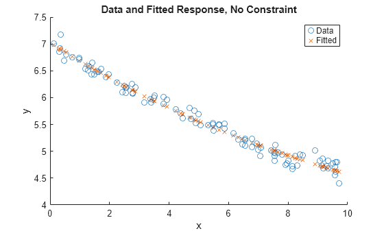
figure
scatter(xdata,ydata)
hold on
scatter(xdata,fitfun(sol2,xdata),"x")
hold off
xlabel("x")
ylabel("y")
legend("Data","Fitted with Constraint")
title("Data and Fitted Response with Constraint")