Nonlinear Least-Squares, Problem-Based
This example shows how to perform nonlinear least-squares curve fitting using the Problem-Based Optimization Workflow.
Model
The model equation for this problem is
where , , , and are the unknown parameters, is the response, and is time. The problem requires data for times tdata and (noisy) response measurements ydata. The goal is to find the best and , meaning those values that minimize
Sample Data
Typically, you have data for a problem. In this case, generate artificial noisy data for the problem. Use A = [1,2] and r = [-1,-3] as the underlying values, and use 200 random values from 0 to 3 as the time data. Plot the resulting data points.
rng default % For reproducibility
A = [1,2];
r = [-1,-3];
tdata = 3*rand(200,1);
tdata = sort(tdata); % Increasing times for easier plotting
noisedata = 0.05*randn(size(tdata)); % Artificial noise
ydata = A(1)*exp(r(1)*tdata) + A(2)*exp(r(2)*tdata) + noisedata;
plot(tdata,ydata,"r*")
xlabel("t")
ylabel("Response")
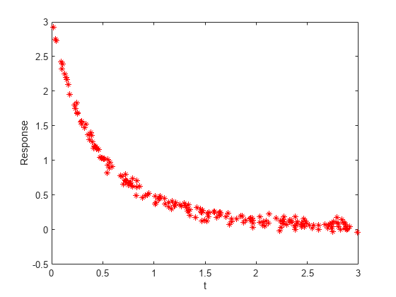
The data are noisy. Therefore, the solution probably will not match the original parameters A and r very well.
Problem-Based Approach
To find the best-fitting parameters A and r, first define optimization variables with those names.
A = optimvar("A",2);
r = optimvar("r",2);
Create an expression for the objective function, which is the sum of squares to minimize.
fun = A(1)*exp(r(1)*tdata) + A(2)*exp(r(2)*tdata);
obj = sum((fun - ydata).^2);
Create an optimization problem with the objective function obj.
lsqproblem = optimproblem("Objective",obj);For the problem-based approach, specify the initial point as a structure, with the variable names as the fields of the structure. Specify the initial A = [1/2,3/2] and the initial r = [-1/2,-3/2].
x0.A = [1/2,3/2];
x0.r = [-1/2,-3/2];
Review the problem formulation.
show(lsqproblem)
  OptimizationProblem :

	Solve for:
       A, r

	minimize :
       sum(arg6)

       where:

           arg5 = extraParams{3};
           arg6 = (((A(1) .* exp((r(1) .* extraParams{1}))) + (A(2) .* exp((r(2) .* extraParams{2})))) - arg5).^2;

       extraParams
Problem-Based Solution
Solve the problem.
[sol,fval] = solve(lsqproblem,x0)
Solving problem using lsqnonlin.

Local minimum found.

Optimization completed because the size of the gradient is less than
the value of the optimality tolerance.

<stopping criteria details>
sol = struct with fields:
    A: [2×1 double]
    r: [2×1 double]
fval =
0.4724
Plot the resulting solution and the original data.
figure
responsedata = evaluate(fun,sol);
plot(tdata,ydata,"r*",tdata,responsedata,"b-")
legend("Original Data","Fitted Curve")
xlabel("t")
ylabel("Response")
title("Fitted Response")

The plot shows that the fitted data match the original noisy data fairly well.
See how closely the fitted parameters match the original parameters A = [1,2] and r = [-1,-3].
disp(sol.A)
    1.1615
    1.8629
disp(sol.r)
   -1.0882
   -3.2256
The fitted parameters are off by about 15% in A and 8% in r.
Unsupported Functions Require fcn2optimexpr
If your objective function is not composed of elementary functions, you must convert the function to an optimization expression using fcn2optimexpr. See Convert Nonlinear Function to Optimization Expression. For the present example:
fun = @(A,r) A(1)*exp(r(1)*tdata) + A(2)*exp(r(2)*tdata);
response = fcn2optimexpr(fun,A,r);
obj = sum((response - ydata).^2);
The remainder of the steps in solving the problem are the same. The only other difference is in the plotting routine, where you call response instead of fun:
responsedata = evaluate(response,sol);
For the list of supported functions, see Supported Operations for Optimization Variables and Expressions.