Predict Engine Torque Using Two-Stage Modeling
This two-stage modeling example shows you how to create a statistical model of an engine that predicts the engine brake torque as a function of spark, engine speed, load, and air/fuel ratio. One-stage modeling fits a model to all the data in one process, without accounting for the structure of the data. When data has an obvious hierarchical structure (as here), two-stage modeling is better suited to the task.
The usual way for collecting brake torque data is to fix engine speed, load, and air/fuel ratio within each test and sweep the spark angle across a range of angles. For this experimental setup, there are two sources of variation. The first source is variation within tests when the spark angle is changed. The second source of variation is between tests when the engine speed, load, and air/fuel ratio are changed. The variation within a test is called local, and the variation between tests, global. Two-stage modeling estimates the local and global variation separately by fitting local and global models in two stages. A local model is fitted to each test independently. The results from all the local models are used to fit global models across all the global variables. Once the global models have been estimated, they can be used to estimate the local models' coefficients for any speed, load, and air/fuel ratio. The relationship between the local and global models is shown in this block diagram.
To get started with two-stage modeling, follow these workflow steps.
Workflow Steps | Description |
|---|---|
Set up your local and global models, select data for modeling, and specify a response to be modeled. | |
Start the toolbox and load and view some data for modeling. | |
Examine the model fit to the data by looking at the local, global, and two-stage response models. | |
Export your completed model, for example, for use in the CAGE part of the toolbox for calibrating. | |
Useful methods for creating multiple different models to search for the best possible fit to the data. |
Open the App and Load Data
In MATLAB®, on the Apps tab, in the Automotive group, click MBC Model Fitting.
If you have never used the toolbox before, the User Information dialog box may appear. If you want, you can fill in any or all of the fields: your name, company, department, and contact information, or you can click Cancel. The user information is used to tag comments and actions so that you can track changes in your files (it does not collect information for MathWorks®).
When you finish with the User Information dialog box, click OK.
The Model Browser window appears.
Load the example data Excel® file holliday:
In the Model Browser, click Import data.
In the Select data file to import dialog box, open the file
holliday. The file is in the<matlabroot>/toolbox/mbc/mbctrainingThe Data Editor opens.
View plots of the data in the Data Editor by selecting variables and tests in the lists on the left side. Have a look through the data to get an idea of the shape of curve formed by plotting torque against spark.
Use the editor to prepare your data before model fitting.
Close the Data Editor to accept the data and return to the Model Browser.
This data is from Holliday, T., “The Design and Analysis of Engine Mapping Experiments: A Two-Stage Approach,” Ph.D. thesis, University of Birmingham, 1995.
Set Up the Model
Specifying Model Inputs
You can use the imported data to create a statistical model of an automobile engine that predicts the torque generated by the engine as a function of spark angle and other variables.
In the Model Browser, click Fit Models.
In the Fit Models dialog box, observe that the
Data Objectyou imported is selected in the Data set list.Click the Two-Stage test plan icon in the Template pane.
In the Inputs and Responses pane, select data channels to use for the responses you want to model.
The model you are building is intended to predict the torque generated by an engine as a function of spark angle at a specified operating point defined by the engine speed, air/fuel ratio, and load. The input to the local model is therefore the spark angle, and the response is torque.
The inputs to the global model are the variables that determine the operating point of the system being modeled. In this example, the operating point of the engine is determined by the engine speed in revolutions per minute (rpm - often called N), load (L), and air/fuel ratio (afr).
Select
sparkin the Data channels list and click the button to add it to the Local inputs list.Select
n,load, andafrin the Data channels list and click the button to add them to the Global inputs list.
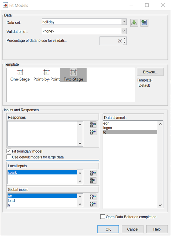
Leave the responses empty, and click OK.
The default name of the new test plan, Two-Stage, appears in the Model
Browser tree, in the All Models pane.
In this window, the left pane, All Models, shows the hierarchy of the models currently built in a tree. At the start, only one node, the project, is in the tree. As you build models, they appear as child nodes of the project. The right panes change, depending on the tree node selected. You navigate to different views by selecting different nodes in the model tree.
Setting Up the Response Model
To achieve the best fit to torque/spark sweeps, you need to change the local model type from the default. The type of a local model is the shape of curve used to fit the test data, for example, quadratic, cubic, or polynomial spline curves. In this example, you use polynomial spline curves to fit the test data. A spline is a curve made up of pieces of polynomial, joined smoothly together. The points of the joins are called knots. In this case, there is only one knot. These polynomial spline curves are useful for torque/spark models, where different curvature is required above and below the maximum.
To change from the default models and specify polynomial spline as the local model type,
In the Model Browser, select the test plan node
Two-Stage, and in the Common Tasks pane, click Fit Models. A dialog box asks if you want to change all the test plan models. Click Yes.In the Fit Models Wizard, click Next to continue using the currently selected data.
The next screen shows the model inputs you already selected. Click Next.
To choose the response, on the Response Models screen, select
tqand click Add.Edit the Local model type by clicking Set Up.
The Local Model Setup dialog box appears.
Select
Polynomial splinefrom the Local model class list.Edit the Spline Order Below knot to
2, and leave Above knot set to2.Click OK to close the dialog box.
Select
Maximumunder Datum. Only certain model types with a clearly defined maximum or minimum can support datum models.Click Finish.
The Model Browser calculates local and global models using the test plan models you just set up.
Notice that the new name of the local model class, PS (for
polynomial spline) 2,2 (for spline order above and below knot) now
appears on a new node in the tree in the All Models pane, called
PS22.
Verify the Model
Verifying the Local Model
The first step is to check that the local models agree well with the data:
If necessary, select
PS22(the local node) on the Model Browser tree.The Local Model view appears, displaying the local model fitting the torque/spark data for the first test and diagnostic statistics that describe the fit. The display is flexible in that you can drag, open, and close the divider bars separating the regions of the screen to adjust the view.
View local model plots and statistics. The Sweep Plot shows the data being fitted by the model (blue dots) and the model itself (line). The red spot shows the position of the polynomial spline knot, at the datum (maximum) point.
Look for problem tests with the RMSE Plots. The plot shows the standard errors of all the tests, both overall and by response feature. Navigate to a test of interest by double-clicking a point in the plot to select the test in the other plots in the local model view.
In the Diagnostic Statistics plot pane, click the Y-axis factor pop-up menu and select
Studentized residuals.Scroll through local models test by test using the Test arrows at the top left, or by using the Select Test button.
Select Test 588. You see a data point outlined in red. This point has automatically been flagged as an outlier.
Right-click the plot and select Remove Outliers. Observe that the model is refitted without the outlier.
Both plots have right-click pop-up menus offering various options such as removing and restoring outliers and confidence intervals. Clicking any data point marks it in red as an outlier.
You can use the Test Notes pane to record information on particular tests. Each test has its own notes pane. The test numbers of data points with notes recorded against them are colored in the global model plots, and you can choose the color using the Test Number Color button in the Test Notes pane. Quickly locate tests with notes by clicking Select Test.
Verifying the Global Model
The next step is to check through the global models to see how well they fit the data:
Expand the
PS22local node on the Model Browser tree by clicking the plus sign (+) to the left of the icon. Under this node are four response features of the local model. Each of these is a feature of the local model of the response, which is torque.Select the first of the global models,
knot.You see a dialog box asking if you want to update fits, because you removed an outlier at the local level. Click Yes.
The Response Feature view appears, showing the fit of the global model to the data for
knot. Fitting the local model is the process of finding values for these coefficients or response features. The local models produce a value ofknotfor each test. These values are the data for the global model forknot. The data for each response feature come from the fit of the local model to each test.Use the plots to assess model fits.
Select the response feature
Bhigh_2. One outlier is marked. Points with an absolute studentized residual value of more than 3 are automatically suggested as outliers (but included in the model unless you take action). You can use the right-click menu to remove suggested outliers (or any others you select) in the same way as from the Local Model plots. Leave this one. If you zoom in on the plot (Shift-click-drag or middle-click-drag) you can see the value of the studentized residual of this point more clearly. Double-click to return to the previous view.Select the other response features in turn:
maxandBlow 2. You see thatBlow 2has a suggested outlier with a very large studentized residual; it is a good distance away from all the other data points for this response feature. All the other points are so clustered that removing this one could greatly improve the fit of the model to the remaining points, so remove it.
Creating the Two-Stage Model
Recall how two-stage models are constructed: two-stage modeling partitions the variation separately between tests and within tests, by fitting local and global models separately. A model is fitted to each test independently (local models). These local models are used to generate global models that are fitted across all tests.
For each sweep (test) of spark against torque, you fit a local model. The local model in
this case is a spline curve, which has the fitted response features of
knot, max, Bhigh_2, and
Blow_2. The result of fitting a local model is a value for
knot (and the other coefficients) for each test. The global model for
knot is fitted to these values (that is, the knot
global model fits knot as a function of the global variables). The
values of knot from the global model (along with the other global models) are then used to
construct the two-stage model.
The global models are used to reconstruct a model for the local response (in this case, torque) that spans all input factors. This is the two-stage model across the whole global space, derived from the global models.
After you are satisfied with the fit of the local and global models, it is time to construct a two-stage model from them.
Return to the Local Model view by clicking the local node
PS22in the Model Browser tree.To create a two-stage model, click Create Two-Stage in the Common Tasks pane.
Comparing the Local Model and the Two-Stage Model
Now the plots in the Local Model view show two lines fitted to the test data. Scroll though the tests using the left/right arrows or the Select Test button at the top left. The plots now show the fit of the two-stage model for each test (green circles and line), compared with the fit of the local model (blue line) and the data (blue dots). Zoom in on points of interest by Shift-click-dragging or middle-click-dragging. Double-click to return the plot to the original size.
Compare how close the two-stage model fit is to both the data and the local fit for each test.
Notice that the local model icon has changed (from the local
 icon showing a house, to a two-stage icon
  showing a house and a globe) to indicate that a two-stage model
has been calculated.
showing a house and a globe) to indicate that a two-stage model
has been calculated.
Response Node
Click the Response node (tq) in the Model Browser tree.
Now at the Response node in the Model Browser tree (tq), which was
previously blank, you see plots showing you the fit of the two-stage model to the data. You can
scroll through the tests, using the arrows at top left, to view the two-stage model against the
data for groups of tests.
You have now completed setting up and verifying a two-stage model.
Export the Model
All models created in the Model Browser are exported using the File menu. A model can be exported to the MATLAB workspace, to CAGE, or to a Simulink® model.
Click the
tqnode in the model tree.Choose File > Export Models. The Export Model dialog box appears.
For the Export to parameter, select the
Simulink,Workspace, orCAGE.Click OK to export the models.
To import models into CAGE to create calibrations, use the CAGE Import Tool instead for more flexibility.
Create Multiple Models to Compare
Methods for Creating More Models
After you have fitted and examined a single model, you normally want to create more models to search for the best fit. You can create individual new models or use the Create Alternatives common task to create a selection of models at once, or create a template to save a variety of model settings for reuse.
To use the Model Template dialog box to quickly create a selection of different child nodes to compare, click Create Alternatives in the Common Tasks pane. The following exercises show you examples of these processes.
Creating New Local Models
To follow these examples, you need to create the initial models.
As an example, select the
tqresponse node and click New Local Model in the Common Tasks pane.The Local Model Setup dialog box appears.
Select a
Polynomial Spline, and edit the spline order to3below the knot and2above. Click OK.A new set of local models (and associated response feature models) is calculated.
Return to the parent
tqresponse node , and click New Local Model again, in the Common Tasks pane.Select a
Polynomialwith an order of2in the Local Model Setup dialog box. Click OK.A new set of local models and response feature models is calculated.
Now you have three alternative local models to compare: two polynomial splines (order 3,2 and order 2,2) and a polynomial (order 2), as shown.
You can select the alternative local models in turn and compare their statistics. For an example, follow these steps:
Select the new local model node
PS32.Select test
587in the Test edit box.In the Local statistics pane, observe the value of RMSE (root mean squared error) for the current (ith) test.
The RMSE value is our basic measure of how closely a model fits some data, which measures the average mismatch between each data point and the model. This is why you should look at the RMSE values as your first tool to inspect the quality of the fit — high RMSE values can indicate problems.
Now select the local model node
POLY2and see how the value ofRMSEchanges.Observe that the shape of the torque/spark sweep for this test is better suited to a polynomial spline model than a polynomial model. The curve is not symmetrical because curvature differs above and below the maximum (marked by the red cross at the datum). This explains why the value of
RMSEis much lower forPS32(the polynomial spline) than for thePOLY2(polynomial) for this test. The polynomial spline is a better fit for the current test.Look through some other tests and compare the values of
RMSEfor the different local models. To choose the most suitable local model you must decide which fits the majority of tests better, as there are likely to be differences among best fit for different tests.To help you quickly identify which local models have the highest RMSE, indicating problems with the model fit, check the RMSE Plots.
Use the plot to help you identify problem tests. Use the drop-down menus to change the display. For example, select
s_knotto investigate the error values for knot (MBT), orRMSEto look at overall error.You can navigate to a test of interest from the RMSE Plots by double-clicking a point in the plot to select the test in the other plots.
Look at the value of
Local RMSEreported in the Pooled Statistics pane on the right (this is pooled between all tests). Now switch between thePOLY2and thePS32local models again and observe how this value changes.You can compare these values directly by selecting the parent
tqresponse node, when the Local RMSE is reported for each child local model in the list at the bottom.When all child models have a two-stage model calculated, you can also compare two-stage values of RMSE here. Remember, you can see statistics to compare the list of child models of the response node in this bottom list pane.
When comparing models, look for lower RMSE values to indicate better fits. However, remember that a model that interpolates between all the points can have an RMSE of zero but be useless for predicting between points. Always use the graphical displays to visually examine model fits and beware of “overfitting” — chasing points at the expense of prediction quality. You will return to the problem of overfitting in a later section when you have two-stage models to compare.
Adding New Response Features
Recall that two-stage models are made up of local models and global models. The global models are fitted to the response features of the local models. The response features available are specific to the type of local model. You can add different response features to see which combination of response features makes the best two-stage model as follows:
Select the local model node
PS32.Select File > New Response Feature.
A dialog box appears with a list of available response features.
Select
f(x+datum)from the list and enter -10in the Value edit box. Click OK.A new response feature called
FX_less10is added under thePS32local model. Recall that the datum marks the maximum, in this case maximum torque. The spark angle at maximum torque is referred to as maximum brake torque (MBT). You have defined this response feature (f(x+datum)) to measure the value of the model (torque) at (-10 + MBT) for each test. It can be useful to use a response feature like this to track a value such as maximum brake torque (MBT) minus 10 degrees of spark angle. This response feature is not an abstract property of a curve, so engineering knowledge can then be applied to increase confidence in the models.Select the local node
PS32, and click Create Two-Stage in the Common Tasks pane. The Model Selection window opens, because you now need to choose 5 of the 6 response features to form the two-stage model.In the Model Selection window, observe four possible two-stage models in the Model List. This is because you added a sixth response feature. Only five (which must include
knot) are required for the two-stage model, so you can see the combinations available and compare them. Note that not all combinations of five response features can completely describe the shape of the curve for the two-stage model, so only the possible alternatives are shown.Close the Model Selection window and click Yes to accept one of the models as best.
Notice that the response features chosen to calculate the two-stage model are highlighted in blue, and the unused response feature is not highlighted.
Select the
tqresponse node to see a comparison of the statistics of both two-stage models (your originalPS22and the newPS32).Remember that the
POLY2local model has no two-stage model yet; no two-stage statistics are reported forPOLY2in the bottom list pane. You cannot fully compare the two-stage models until every local model in the test plan has a two-stage model calculated.To calculate the two-stage model for
POLY2, in the Common Tasks pane, click Create Two-Stage.
Comparing Models
Now you have three two-stage models. Select the
tqresponse node and look at the statistics, particularly Local RMSE and Two-Stage RMSE reported in the list of child models at the bottom.Look for lower RMSE values to indicate better fits.
Look for lower PRESS RMSE values to indicate better fits without overfitting. PRESS RMSE is a measure of the predictive power of your models.
It is useful to compare PRESS RMSE with RMSE as this may indicate problems with overfitting. RMSE is minimized when the model gets close to each data point; “chasing” the data will therefore improve RMSE. However, chasing the data can sometimes lead to strong oscillations in the model between the data points; this behavior can give good values of RMSE but is not representative of the data and will not give reliable prediction values where you do not already have data. The PRESS RMSE statistic guards against this by testing how well the current model would predict each of the points in the data set (in turn) if they were not included in the regression. To get a small PRESS RMSE usually indicates that the model is not overly sensitive to any single data point.
Look for lower T^2 values. A large T^2 value indicates that there is a problem with the response feature models.
Look for large negative log likelihood values to indicate better fits.
To compare all three two-stage models simultaneously, select Model > Selection Window. Here you can see the same statistics to compare the models in the bottom list, but you can also make use of a variety of views to look for the best fit:
You can plot the models simultaneously on the Tests, Residuals and Cross Section views (Shift- or Ctrl-click to select models in the list)
You can view each model in the Response Surface view as a surface; movie, contour or multiline plot, and as a table
You can select a model and click Assign Best in the Model Selection window, or double-click a model to assign it as best.
When you close the Model Selection window and return to the Model Browser, the model you selected as best is copied to the parent response node,
tq.
Creating New Global Models
In this example, you have not yet searched for the best global model types. You would normally do this before creating and comparing two-stage models. For the purpose of this tutorial, you have already created two-stage models and used RMSE to help you identify better models. The principle is the same at each level in the model tree: add new child models and choose the best. You can create any number of child nodes to search for the best global model fit for each response feature in your tree.
Select the local node
POLY2.To create a selection of alternatives for each response feature node, in the Common Tasks pane, click Build Global Models.
In the Model Template dialog box, click New, then click OK.
Observe the default list of a variety of model types, then click OK. It is worth trying the default model settings for a quick exploration of the trends in the data.
In the Model Selection dialog box, leave the default selection criterion for automatically choosing the best child node, and click OK.
The toolbox builds the models and selects the best using your selection criteria.
Note
The toolbox automatically builds models in parallel if you have Parallel Computing Toolbox™.
Assess all the fits in the Alternative Models list in case you want to choose an alternative as a better fit.
Notice that the child node model assigned as best is highlighted in blue in the Alternative Models list and the model tree. The local node has changed from the two-stage icon back to the local model icon (a red house). This is because you have changed the response feature models, and so you need to recalculate the two-stage model using the new global models for the response features.
When you have chosen best global models for all your response features, you need to recalculate the two-stage model.
When you have chosen a best model among alternatives, it can be useful to clean up the rejected models by selecting Delete Alternatives in the Common Tasks pane. You can also select File > Clean Up Tree. This deletes all rejected child models where best models have been chosen; only the child nodes selected as best remain.
You can use the Model Template dialog box to create and save templates of model types you often want to build. Creating a template containing a list of all the models you want is an efficient way to quickly build a selection of alternative model child nodes for many global models. Use these techniques to find models well suited to the data for each of your global models.