amd

Approximate minimum degree permutation

Syntax

P = amd(A)
P = amd(A,opts)


Description

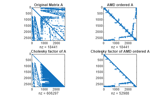
P = amd(A) returns the approximate minimum degree permutation vector for the sparse matrix C = A + A'. The Cholesky factorization of C(P,P) or A(P,P) tends to be sparser than that of C or A. The amd function tends to be faster than symamd, and also tends to return better orderings than symamd. Matrix A must be square. If A is a full matrix, then amd(A) is equivalent to amd(sparse(A)).

P = amd(A,opts) allows additional options for the reordering. The opts input is a structure with the two fields shown below. You only need to set the fields of interest:

• dense — A nonnegative scalar value that indicates what is considered to be dense. If A is n-by-n, then rows and columns with more than max(16,(dense*sqrt(n))) entries in A + A' are considered to be "dense" and are ignored during the ordering. MATLAB^® software places these rows and columns last in the output permutation. The default value for this field is 10.0 if this option is not present.

• aggressive — A scalar value controlling aggressive absorption. If this field is set to a nonzero value, then aggressive absorption is performed. This is the default if this option is not present.

MATLAB software performs an assembly tree post-ordering, which is typically the same as an elimination tree post-ordering. It is not always identical because of the approximate degree update used, and because “dense” rows and columns do not take part in the post-order. It well-suited for a subsequent chol operation, however, If you require a precise elimination tree post-ordering, you can use the following code:

P = amd(S);
C = spones(S)+spones(S'); 
[ignore, Q] = etree(C(P,P));
P = P(Q);

If S is already symmetric, omit the second line, C = spones(S)+spones(S').

Examples

Effect of Preordering on Sparsity of Cholesky Factors

Compute the Cholesky factor of a matrix before and after it is ordered using amd to examine the effect on sparsity.

Load the barbell graph sparse matrix and add a sparse identity matrix to it to ensure it is positive definite. Compute two Cholesky factors: one of the original matrix and one of the original matrix preordered with amd.

load barbellgraph.mat
A = A+speye(size(A)); 
p = amd(A);
L = chol(A,'lower');
Lp = chol(A(p,p),'lower');

Plot the sparsity patterns of all four matrices. The Cholesky factor obtained from the preordered matrix is much sparser compared to the factor of the matrix in its natural ordering.

figure
subplot(2,2,1)
spy(A)
title('Original Matrix A')
subplot(2,2,2) 
spy(A(p,p))
title('AMD ordered A')
subplot(2,2,3) 
spy(L)
title('Cholesky factor of A')
subplot(2,2,4) 
spy(Lp)
title('Cholesky factor of AMD ordered A')

References

[1] Amestoy, Patrick R., Timothy A. Davis, and Iain S. Duff. “Algorithm 837: AMD, an Approximate Minimum Degree Ordering Algorithm.” ACM Transactions on Mathematical Software 30, no. 3 (September 2004): 381–388. https://doi.org/10.1145/1024074.1024081.

Extended Capabilities

Thread-Based Environment

Run code in the background using MATLAB® backgroundPool or accelerate code with Parallel Computing Toolbox™ ThreadPool.

This function fully supports thread-based environments. For more information, see Run MATLAB Functions in Thread-Based Environment.