Solve System of ODEs with Multiple Initial Conditions
This example compares two techniques to solve a system of ordinary differential equations with multiple sets of initial conditions. The techniques are:
Use a
for-loop to perform several simulations, one for each set of initial conditions. This technique is simple to use but does not offer the best performance for large systems.Vectorize the ODE function to solve the system of equations for all sets of initial conditions simultaneously. This technique is the faster method for large systems but requires rewriting the ODE function so that it reshapes the inputs properly.
The equations used to demonstrate these techniques are the well-known Lotka-Volterra equations, which are first-order nonlinear differential equations that describe the populations of predators and prey.
Problem Description
The Lotka-Volterra equations are a system of two first-order, nonlinear ODEs that describe the populations of predators and prey in a biological system. Over time, the populations of the predators and prey change according to the equations
The variables in these equations are
is the population size of the prey
is the population size of the predators
is time
, , , and are constant parameters that describe the interactions between the two species. This example uses the parameter values , , and .
For this problem, the initial values for and are the initial population sizes. Solving the equations then provides information about how the populations change over time as the species interact.
Solve Equations with One Initial Condition
To solve the Lotka-Volterra equations in MATLAB®, write a function that encodes the equations, specify a time interval for the integration, and specify the initial conditions. Then you can use one of the ODE solvers, such as ode45, to simulate the system over time.
A function that encodes the equations is
function dpdt = lotkaODE(t,p)
% LOTKA Lotka-Volterra predator-prey model
delta = 0.02;
beta = 0.01;

dpdt = [p(1) .* (1 - beta*p(2));
        p(2) .* (-1 + delta*p(1))];
end
(This function is included as a local function at the end of the example.)
Since there are two equations in the system, dpdt is a vector with one element for each equation. Also, the solution vector p has one element for each solution component: p(1) represents in the original equations, and p(2) represents in the original equations.
Next, specify the time interval for integration as and set the initial population sizes for and to 50.
t0 = 0;
tfinal = 15;
p0 = [50; 50];
Solve the system with ode45 by specifying the ODE function, the time span, and the initial conditions. Plot the resulting populations versus time.
[t,p] = ode45(@lotkaODE,[t0 tfinal],p0);
plot(t,p)
title('Predator/Prey Populations Over Time')
xlabel('t')
ylabel('Population')
legend('Prey','Predators')
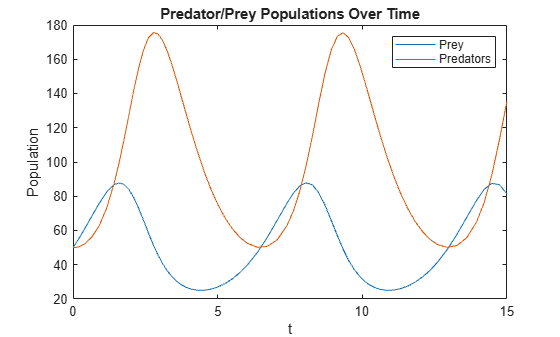
Since the solutions exhibit periodicity, plot the solutions against each other in a phase plot.
plot(p(:,1),p(:,2))
title('Phase Plot of Predator/Prey Populations')
xlabel('Prey')
ylabel('Predators')
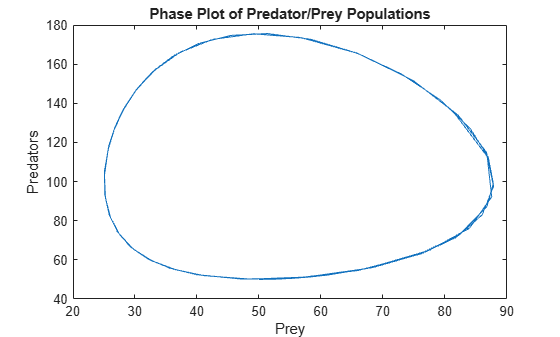
The resulting plots show the solution for the given initial population sizes. To solve the equations for different initial population sizes, change the values in p0 and rerun the simulation. However, this method only solves the equations for one initial condition at a time. The next two sections describe techniques to solve for many different initial conditions.
Method 1: Compute Multiple Initial Conditions with for-loop
The simplest way to solve a system of ODEs for multiple initial conditions is with a for-loop. This technique uses the same ODE function as the single initial condition technique, but the for-loop automates the solution process.
For example, you can hold the initial population size for constant at 50, and use the for-loop to vary the initial population size for between 10 and 400. Create a vector of population sizes for y0, and then loop over the values to solve the equations for each set of initial conditions. Plot a phase plot with the results from all iterations.
y0 = 10:10:400;
for k = 1:length(y0)
    [t,p] = ode45(@lotkaODE,[t0 tfinal],[50 y0(k)]);
    plot(p(:,1),p(:,2))
    hold on
end
title('Phase Plot of Predator/Prey Populations')
xlabel('Prey')
ylabel('Predators')
hold off
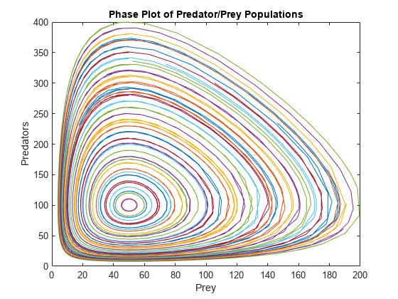
The phase plot shows all of the computed solutions for the different sets of initial conditions.
Method 2: Compute Multiple Initial Conditions with Vectorized ODE Function
Another method to solve a system of ODEs for multiple initial conditions is to rewrite the ODE function so that all of the equations are solved simultaneously. The steps to do this are:
Provide all of the initial conditions to
ode45as a matrix. The size of the matrix iss-by-n, wheresis the number of solution components andnis the number of initial conditions being solved for. Each column in the matrix then represents one complete set of initial conditions for the system.The ODE function must accept an extra input parameter for
n, the number of initial conditions.Inside the ODE function, the solver passes the solution components p as a column vector. The ODE function must reshape the vector into a matrix with size
s-by-n. Each row of the matrix then contains all of the initial conditions for each variable.The ODE function must solve the equations in a vectorized format, so that the expression accepts vectors for the solution components. In other words,
f(t,[y1 y2 y3 ...])must return[f(t,y1) f(t,y2) f(t,y3) ...].Finally, the ODE function must reshape its output back into a vector so that the ODE solver receives a vector back from each function call.
If you follow these steps, then the ODE solver can solve the system of equations using a vector for the solution components, while the ODE function reshapes the vector into a matrix and solves each solution component for all of the initial conditions. The result is that you can solve the system for all of the initial conditions in one simulation.
To implement this method for the Lotka-Volterra system, start by finding the number of initial conditions n, and then form a matrix of initial conditions.
n = length(y0);
p0_all = [50*ones(n,1) y0(:)]';
Next, rewrite the ODE function so that it accepts n as an input. Use n to reshape the solution vector into a matrix, then solve the vectorized system and reshape the output back into a vector. A modified ODE function that performs these tasks is
function dpdt = lotkasystem(t,p,n)
%LOTKA  Lotka-Volterra predator-prey model for system of inputs p.
delta = 0.02;
beta = 0.01;

% Change the size of p to be: Number of equations-by-number of initial
% conditions.
p = reshape(p,[],n);

% Write equations in vectorized form.
dpdt = [p(1,:) .* (1 - beta*p(2,:));
        p(2,:) .* (-1 + delta*p(1,:))];

% Linearize output.
dpdt = dpdt(:);
end
Solve the system of equations for all of the initial conditions using ode45. Since ode45 requires the ODE function to accept two inputs, use an anonymous function to pass in the value of n from the workspace to lotkasystem.
[t,p] = ode45(@(t,p) lotkasystem(t,p,n),[t0 tfinal],p0_all);
Reshape the output vector into a matrix with size (numTimeSteps*s)-by-n. Each column of the output p(:,k) contains the solutions for one set of initial conditions. Plot a phase plot of the solution components.
p = reshape(p,[],n);
nt = length(t);
for k = 1:n
    plot(p(1:nt,k),p(nt+1:end,k))
    hold on
end
title('Predator/Prey Populations Over Time')
xlabel('t')
ylabel('Population')
hold off
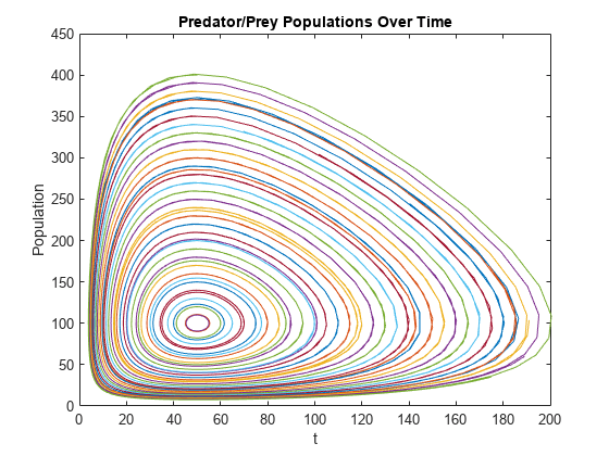
The results are comparable to those obtained by the for-loop technique. However, there are some properties of the vectorized solution technique that you should keep in mind:
The calculated solutions can be slightly different than those computed from a single initial input. The difference arises because the ODE solver applies norm checks to the entire system to calculate the size of the time steps, so the time-stepping behavior of the solution is slightly different. The change in time steps generally does not affect the accuracy of the solution, but rather which times the solution is evaluated at.
For stiff ODE solvers (
ode15s,ode23s,ode23t,ode23tb) that automatically evaluate the numerical Jacobian of the system, specifying the block diagonal sparsity pattern of the Jacobian using theJPatternoption ofodesetcan improve the efficiency of the calculation. The block diagonal form of the Jacobian arises from the input reshaping performed in the rewritten ODE function.
Compare Timing Results
Time each of the previous methods using timeit. The timing for solving the equations with one set of initial conditions is included as a baseline number to see how the methods scale.
% Time one IC
baseline = timeit(@() ode45(@lotkaODE,[t0 tfinal],p0),2);

% Time for-loop
for k = 1:length(y0)
    loop_timing(k) = timeit(@() ode45(@lotkaODE,[t0 tfinal],[50 y0(k)]),2);
end
loop_timing = sum(loop_timing);

% Time vectorized fcn
vectorized_timing = timeit(@() ode45(@(t,p) lotkasystem(t,p,n),[t0 tfinal],p0_all),2);
Create a table with the timing results. Multiply all of the results by 1e3 to express the times in milliseconds. Include a column with the time per solution, which divides each time by the number of initial conditions being solved for.
TimingTable = table(1e3.*[baseline; loop_timing; vectorized_timing], ...
    1e3.*[baseline; loop_timing/n; vectorized_timing/n],...
    'VariableNames',{'TotalTime (ms)','TimePerSolution (ms)'},'RowNames', ...
    {'One IC','Multi ICs: For-loop', 'Mult ICs: Vectorized'})
TimingTable=3×2 table
                            TotalTime (ms)    TimePerSolution (ms)
                            ______________    ____________________

    One IC                     0.11058               0.11058
    Multi ICs: For-loop         4.2562               0.10641
    Mult ICs: Vectorized        1.3758              0.034394
The TimePerSolution column shows that the vectorized technique is the fastest of the three methods.
Local Functions
Listed here are the local functions that ode45 calls to calculate the solutions.
function dpdt = lotkaODE(t,p)
% LOTKA Lotka-Volterra predator-prey model
delta = 0.02;
beta = 0.01;

dpdt = [p(1) .* (1 - beta*p(2));
        p(2) .* (-1 + delta*p(1))];
end
%------------------------------------------------------------------
function dpdt = lotkasystem(t,p,n)
%LOTKA  Lotka-Volterra predator-prey model for system of inputs p.
delta = 0.02;
beta = 0.01;

% Change the size of p to be: Number of equations-by-number of initial
% conditions.
p = reshape(p,[],n);

% Write equations in vectorized form.
dpdt = [p(1,:) .* (1 - beta*p(2,:));
        p(2,:) .* (-1 + delta*p(1,:))];

% Linearize output.
dpdt = dpdt(:);
end