Index and View Tall Array Elements
Tall arrays are too large to fit in memory, so it is common to view subsets of the data rather than the entire array. This page shows techniques to extract and view portions of a tall array.
Extract Top Rows of Array
Use the head function
to extract the first rows in a tall array. head does
not force evaluation of the array, so you must use gather to
view the result.
tt = tall(table(randn(1000,1),randn(1000,1),randn(1000,1)))
tt =

  1,000×3 tall table

      Var1        Var2        Var3
    ________    ________    ________

     0.53767      0.6737     0.29617
      1.8339    -0.66911      1.2008
     -2.2588    -0.40032      1.0902
     0.86217     -0.6718     -0.3587
     0.31877     0.57563    -0.12993
     -1.3077    -0.77809     0.73374
    -0.43359     -1.0636     0.12033
     0.34262     0.55298      1.1363
       :           :           :
       :           :           :
t_head = gather(head(tt))
t_head =

  8×3 table

      Var1        Var2        Var3
    ________    ________    ________

     0.53767      0.6737     0.29617
      1.8339    -0.66911      1.2008
     -2.2588    -0.40032      1.0902
     0.86217     -0.6718     -0.3587
     0.31877     0.57563    -0.12993
     -1.3077    -0.77809     0.73374
    -0.43359     -1.0636     0.12033
     0.34262     0.55298      1.1363
Extract Bottom Rows of Array
Similarly, you can use the tail function
to extract the bottom rows in a tall array.
t_tail = gather(tail(tt))
Evaluating tall expression using the Local MATLAB Session:
- Pass 1 of 1: Completed in 0.13 sec
Evaluation completed in 0.22 sec

t_tail =

  8×3 table

      Var1        Var2        Var3
    ________    ________    ________

     -1.5504    0.060152     -1.1751
     0.29075    -0.12658     -0.4544
      -1.513    -0.57716    -0.50611
    -0.72565    -0.30518      1.8037
     -1.0756    -0.48328     -1.0127
      1.5488    -0.31029     -1.2403
    -0.16252    -0.86155     0.26656
     0.32582       -1.22     -1.2078
Indexing Tall Arrays
All tall arrays support parentheses indexing. When you index a tall array using parentheses,
such as T(A) or T(A,B), the result is a new tall array
containing only the specified rows and columns (or variables).
Like most other operations on tall arrays, indexing expressions are not evaluated
immediately. You must use gather to evaluate the indexing operation.
For more information, see Lazy Evaluation of Tall Arrays.
You can perform these types of indexing in the first dimension of a tall array:
B = A(:,…), where:selects all rows inA.B = A(idx,…), whereidxis a tall numeric column vector or non-tall numeric vector.B = A(L,…), whereLis a tall or non-tall logical array of the same height asA. For example, you can use relational operators, such astt(tt.Var1 < 10,:). When you index a tall array with a tall logical array, there are a few requirements. Each of the tall arrays:Must be the same size in the first dimension.
Must be derived from a single tall array.
Must not have been indexed differently in the first dimension.
B = A(P:D:Q,…)orB = A(P:Q,…), whereP:D:QandP:Qare validcolonindexing expressions.head(tt,k)provides a shortcut fortt(1:k,:).tail(tt,k)provides a shortcut fortt(end-k:end,:).
Additionally, the number of subscripts you must specify depends on how many dimensions the array has:
For tall column vectors, you can specify a single subscript such as
t(1:10).For tall row vectors, tall tables, and tall timetables, you must specify two subscripts.
For tall arrays with two or more dimensions, you must specify two or more subscripts. For example, if the array has three dimensions, you can use an expression such as
tA(1:10,:,:)ortA(1:10,:), but not linear indexing expressions such astA(1:10)ortA(:).
Tip
The find function locates nonzero elements in
tall column vectors, and can be useful to generate a vector of indices for elements that
meet particular conditions. For example, k = find(X<0) returns the
linear indices for all negative elements in X.
For example, use parentheses indexing to retrieve the first
ten rows of tt.
tt(1:10,:)
ans =

  10×3 tall table

      Var1        Var2        Var3
    ________    ________    ________

     0.53767      0.6737     0.29617
      1.8339    -0.66911      1.2008
     -2.2588    -0.40032      1.0902
     0.86217     -0.6718     -0.3587
     0.31877     0.57563    -0.12993
     -1.3077    -0.77809     0.73374
    -0.43359     -1.0636     0.12033
     0.34262     0.55298      1.1363
       :           :           :
       :           :           :
Retrieve the last 5 values of the table variable Var1. Tall arrays use lazy
evaluation, meaning they remain unevaluated until calculations are explicitly requested.
While in this unevaluated state, MATLAB® might not know the size of the array or the index of the last value in
Var1. As a result, unknown array values are displayed as
?. To learn more, see Lazy Evaluation of Tall Arrays.
tt_End = tt(end-5:end,'Var1')tt_End =
6×1 tall table
Var1
____
?
?
?
?
?
?
Preview deferred. Learn more.To request evaluation of the tt_End variable, use the
gather function.
gather(tt_End)
ans =

  6×1 table

      Var1
    ________

      -1.513
    -0.72565
     -1.0756
      1.5488
    -0.16252
     0.32582
Retrieve every 100th row from the tall table and request evaluation of the tall array using
the gather function.
gather(tt(1:100:end,:))
Evaluating tall expression using the Local MATLAB Session:
- Pass 1 of 2: Completed in 0.043 sec
- Pass 2 of 2: Completed in 0.049 sec
Evaluation completed in 0.15 sec

ans =

  10×3 table

      Var1         Var2        Var3
    _________    ________    ________

      -1.0501     -1.9184    -0.13863
      0.74472      1.5582      2.4409
     -0.69522    -0.81153     0.97164
    -0.027222      0.6195    -0.30732
       -1.505      2.0547    -0.61177
      0.47717      2.3552     0.62645
      -1.7579     0.15488    -0.90923
      0.82525    0.044202    -0.33881
      0.33116     0.43173    -0.53523
    -0.047305     -1.0763     0.06896
Extract Tall Table Variables
The variables in a tall table or tall timetable are each tall arrays of different
underlying data types. Standard indexing methods of tables and timetables also apply to tall
tables and tall timetables, including the use of timerange, withtol, and vartype.
For example, index a tall table using dot notation T.VariableName to
retrieve a single variable of data as a tall array.
tt.Var1
ans =
1,000×1 tall double column vector
0.5377
1.8339
-2.2588
0.8622
0.3188
-1.3077
-0.4336
0.3426
:
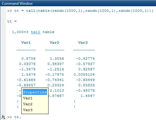
:Use tab completion to look up the variables in a table if you
cannot remember a precise variable name. For example, type tt. and then press Tab.
A menu pops up:
You can also perform multiple levels of indexing. For example,
extract the first 5 elements in the variable Var2.
In this case you must use one of the supported forms of indexing for
tall arrays in the parentheses.
tt.Var2(1:5)
ans =

  5×1 tall double column vector

    0.6737
   -0.6691
   -0.4003
   -0.6718
    0.5756
For more indexing information, see Access Data in Tables or Select Times in Timetable.
Concatenation with Tall Arrays
In order to concatenate two or more tall arrays, as in [A1 A2 A3 …],
each of the tall arrays must be derived from a single tall array and must not have been
indexed differently in the first dimension. Indexing operations include functions such as
vertcat, splitapply, sort,
cell2mat, synchronize,
retime, and so on.
For example, concatenate a few columns from tt to create a new tall
matrix.
[tt.Var1 tt.Var2]
ans =

  1,000×2 tall double matrix

    0.5377    0.6737
    1.8339   -0.6691
   -2.2588   -0.4003
    0.8622   -0.6718
    0.3188    0.5756
   -1.3077   -0.7781
   -0.4336   -1.0636
    0.3426    0.5530
      :         :
      :         :
To combine tall arrays with different underlying datastores, it is recommended that you
use write to write the arrays (or calculation
results) to disk, and then create a single new datastore referencing those locations:
files = {'folder/path/to/file1','folder/path/to/file2'};
ds = datastore(files);
Assignment and Deletion with Tall Arrays
The same subscripting rules apply whether you use indexing to assign or delete elements from a
tall array. Deletion is accomplished by assigning one or more elements to the empty matrix,
[].
“( )” Assignment
You can assign elements into a tall array using the general syntax A(m,n,...) =
B. The tall array A must exist and have a nonempty second
dimension. The first subscript m must be either a colon
: or a tall logical vector. With this syntax, B
can be:
Scalar
A tall array derived from
A(m,…)wheremis the same subscript as above. For example,A(m,1:10).An empty matrix,
[](for deletion)
“.” Assignment
For table indexing using the syntax A.Var1 = B,
the array B must be a tall array with the appropriate
number of rows. Typically, B is derived from existing
data in the tall table. Var1 can be either a new
or existing variable in the tall table.
You cannot assign tall arrays as variables in a regular table, even if the table is empty.
Extract Specified Number of Rows in Sorted Order
Sorting all of the data in a tall array can be an expensive calculation. Most often, only a subset of rows at the beginning or end of a tall array is required to answer questions like “What is the first row in this data by year?”
The topkrows function
returns a specified number of rows in sorted order for this purpose.
For example, use topkrows to extract the top
12 rows sorted in descending order by the second column.
t_top12 = gather(topkrows(tt,12,2))
Evaluating tall expression using the Local MATLAB Session:
Evaluation completed in 0.067 sec

t_top12 =

  12×3 table

      Var1       Var2       Var3
    ________    ______    ________

     -1.0322    3.5699     -1.4689
      1.3312    3.4075     0.17694
    -0.27097    3.1585     0.50127
     0.55095    2.9745       1.382
     0.45168    2.9491     -0.8215
     -1.7115    2.7526     -0.3384
    -0.21317    2.7485      1.9033
    -0.43021    2.7335     0.77616
    -0.59003    2.7304     0.67702
     0.47163    2.7292     0.92099
    -0.47615     2.683    -0.26113
     0.72689    2.5383    -0.57588
Summarize Tall Array Contents
The summary function returns useful information
about each variable in a tall table or timetable, such as the minimum and maximum values of
numeric variables, and the number of occurrences of each category for categorical
variables.
For example, create a tall table for the outages.csv data
set and display the summary information. This data set contains numeric,
datetime, and categorical variables.
fmts = {'%C' '%D' '%f' '%f' '%D' '%C'};
ds = tabularTextDatastore('outages.csv','TextscanFormats',fmts);
T = tall(ds);
summary(T)
Evaluating tall expression using the Local MATLAB Session:
- Pass 1 of 2: Completed in 0.068 sec
- Pass 2 of 2: Completed in 0.073 sec
Evaluation completed in 0.21 sec
T: 1468×6 table
Variables:
Region: categorical (5 categories)
OutageTime: datetime
Loss: double
Customers: double
RestorationTime: datetime
Cause: categorical (10 categories)
Statistics for applicable variables:
NumMissing Min Max Mean
Region 0
OutageTime 0 2002-02-01 12:18 2014-01-15 02:41 2009-07-03 12:49
Loss 604 0 2.3418e+04 563.8885
Customers 328 0 5.9689e+06 1.6693e+05
RestorationTime 29 2002-02-07 16:50 2042-09-18 23:31 2009-07-27 15:47
Cause 0 Return Subset of Calculation Results
Many of the examples on this page use gather to
evaluate expressions and bring the results into memory. However, in
these examples it is also trivial that the results fit in memory,
since only a few rows are indexed at a time.
In cases where you are unsure if the result of an expression
will fit in memory, it is recommended that you use gather(head(X)) or gather(tail(X)).
These commands still evaluate all of the queued calculations, but
return only a small amount of the result that is guaranteed to fit
in memory.
If you are certain that the result of a calculation will not
fit in memory, use write to evaluate the tall
array and write the results to disk instead.
See Also
tall | table | topkrows | head | tail | gather