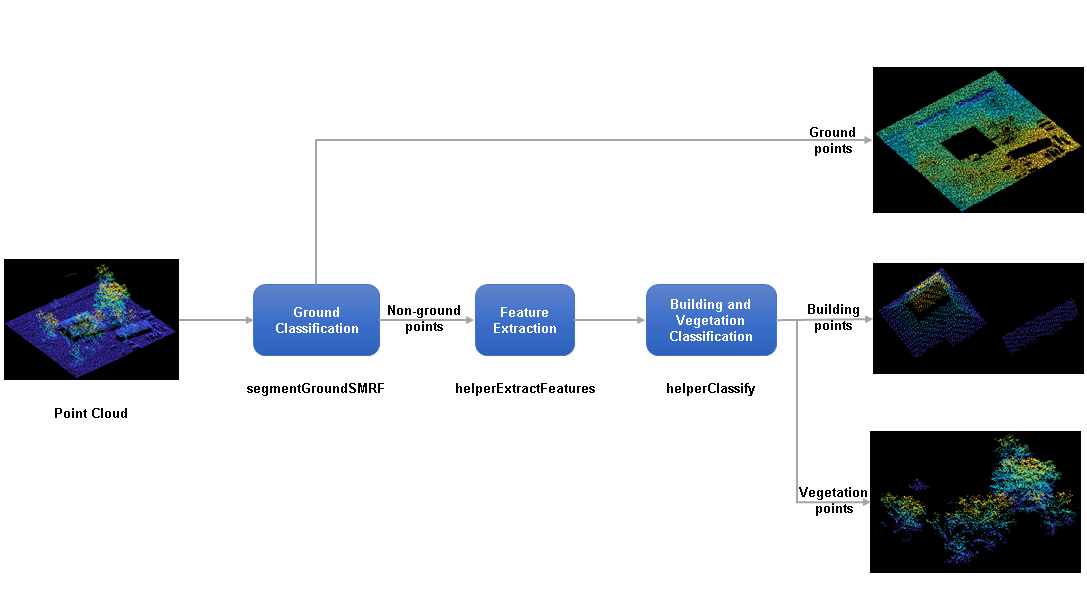
Terrain Classification for Aerial Lidar Data

Open Live Script

This example shows how to segment and classify terrain in aerial lidar data as ground, building, and vegetation. The example uses a LAZ file captured by an airborne lidar system as input. First, classify the point cloud data in the LAZ file into ground and non-ground points. Then, further classify non-ground points into building and vegetation points based on normals and curvature features. This figure provides an overview of the process.

Load and Visualize Data

Load the point cloud data and corresponding ground truth labels from the LAZ file, aerialLidarData.laz, obtained from the Open Topography Dataset [1]. The point cloud consists of various classes, including ground, building, and vegetation. Load the point cloud data and the corresponding ground truth labels into the workspace using the readPointCloud object function of the lasFileReader object. Visualize the point cloud, color-coded according to the ground truth labels, using the pcshow function.

lazfile = fullfile(toolboxdir('lidar'),'lidardata','las','aerialLidarData.laz');
% Read LAZ data from file
lazReader = lasFileReader(lazfile);
% Read point cloud and corresponding ground truth labels
[ptCloud,pointAttributes] = readPointCloud(lazReader, ...
    'Attributes','Classification');
grdTruthLabels = pointAttributes.Classification;
% Visualize the input point cloud with corresponding ground truth labels
figure
pcshow(ptCloud.Location,grdTruthLabels)
title('Aerial Lidar Data with Ground Truth')

Ground Classification

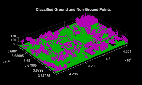
Ground classification is a preprocessing step to segment the input point cloud as ground and non-ground. Segment the data loaded from the LAZ file into ground and non-ground points using the segmentGroundSMRF function.

[groundPtsIdx,nonGroundPtCloud,groundPtCloud] = segmentGroundSMRF(ptCloud);
% Visualize ground and non-ground points in green and magenta, respectively
figure
pcshowpair(nonGroundPtCloud,groundPtCloud)
title('Classified Ground and Non-Ground Points')

Feature Extraction

Extract features from the point cloud using the helperExtractFeatures function. All the helper functions are attached to this example as supporting files. The helper function estimates the normal and curvature values for each point in the point cloud. These features provide underlying structure information at each point by correlating it with the points in its neighborhood.

You can specify the number of neighbors to consider. If the number of neighbors is too low, the helper function overclusters vegetation points. If the number of neighbors is too high, there is no defining boundary between buildings and vegetation, as vegetation points near the building points are misclassified.

neighbors = 10;  
[normals,curvatures,neighInds] = helperExtractFeatures(nonGroundPtCloud, ...
    neighbors);

Building and Vegetation Classification

The helper function uses the variation in normals and curvature to distinguish between buildings and vegetation. The buildings are more planar compared to vegetation, so the change in curvature and the relative difference of normals between neighbors is less for points belonging to buildings. Vegetation points are more scattered, which results in a higher change in curvatures as compared to buildings. The helperClassify function classifies the non-ground points into building and vegetation. The helper function classifies the points as building based on the following criteria:

The curvature of each point must be small, within the specified curvature threshold, curveThresh.
The neighboring points must have similar normals. The cosine similarity between neighboring normals must be greater than the specified normal threshold, normalThresh.

The points that do not satisfy the above criteria are marked as vegetation. The helper function labels the points belonging to vegetation as 1 and building as 2.

% Specify the normal threshold and curvature threshold
normalThresh = 0.85;
curveThresh = 0.02;
% Classify the points into building and vegetation
labels = helperClassify(normals,curvatures,neighInds, ...
    normalThresh,curveThresh);

Extract the building and vegetation class labels from the ground truth label data. As the LAZ file has many classes, you must first isolate the ground, building and vegetation classes. The classification labels are in compliance with the ASPRS standard for LAZ file formats.

Classification Value 2 — Represents ground points
Classification Values 3, 4, and 5 — Represent low, medium, and high vegetation points
Classification Value 6 — Represents building points

Define maskData to extract points belonging to the ground, buildings, and vegetation from the input point cloud.

maskData = grdTruthLabels>=2 & grdTruthLabels<=6;

Modify the ground truth labels of the input point cloud, specified as grdTruthLabels.

% Compress low, medium, and high vegetation to a single value
grdTruthLabels(grdTruthLabels>=3 & grdTruthLabels<=5) = 4;
% Update grdTruthLabels for metrics calculation
grdTruthLabels(grdTruthLabels == 2) = 1;    
grdTruthLabels(grdTruthLabels == 4) = 2;
grdTruthLabels(grdTruthLabels == 6) = 3;

Store the predicted labels acquired from previous classification steps in estimatedLabels.

estimatedLabels = zeros(ptCloud.Count,1);
estimatedLabels(groundPtsIdx) = 1; 
estimatedLabels(labels == 1) = 2;
estimatedLabels(labels == 2) = 3;

Extract the labels belonging to ground, buildings, and vegetation.

grdTruthLabels = grdTruthLabels(maskData);
estimatedLabels = estimatedLabels(maskData);

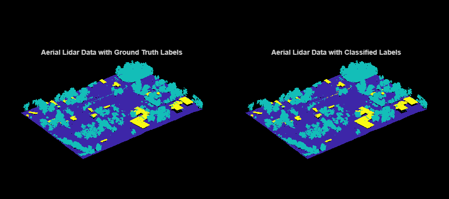
Visualize the terrain with the ground truth and estimated labels.

ptCloud = select(ptCloud,maskData);
hFig = figure('Position',[0 0 900 400]);
axMap1 = subplot(1,2,1,'Color','black','Parent',hFig);
axMap1.Position = [0 0.2 0.5 0.55];
pcshow(ptCloud.Location,grdTruthLabels,'Parent',axMap1)
axis off
title(axMap1,'Aerial Lidar Data with Ground Truth Labels')
axMap2 = subplot(1,2,2,'Color','black','Parent',hFig);
axMap2.Position = [0.5,0.2,0.5,0.55];
pcshow(ptCloud.Location,estimatedLabels,'Parent',axMap2)
axis off
title(axMap2,'Aerial Lidar Data with Classified Labels')

Validation

Validate the classification by computing the total accuracy on the given point cloud along with the class accuracy, intersection-over-union (IoU), and weighted IoU.

confusionMatrix = segmentationConfusionMatrix(estimatedLabels,double(grdTruthLabels));
ssm = evaluateSemanticSegmentation({confusionMatrix}, ...
    {'Ground' 'Vegetation' 'Building'},'Verbose',0);
disp(ssm.DataSetMetrics)

    GlobalAccuracy    MeanAccuracy    MeanIoU    WeightedIoU
    ______________    ____________    _______    ___________

       0.71113          0.54572       0.32094      0.66209

disp(ssm.ClassMetrics)

                  Accuracy      IoU   
                  ________    ________

    Ground        0.72222      0.72222
    Vegetation    0.80549      0.20533
    Building      0.10944     0.035268

References

[1] Starr, Scott. "Tuscaloosa, AL: Seasonal Inundation Dynamics and Invertebrate Communities." National Center for Airborne Laser Mapping, December 1, 2011. OpenTopography (https://doi.org/10.5069/G9SF2T3K)