measureSharpness
Measure spatial frequency response using test chart
Syntax
Description
esfrChart Object
Use an esfrChart object when you want to automatically detect the
slanted-edge regions of interest (ROIs) of an Enhanced or Extended version of the
Imatest® eSFR test chart [1].
sharpnessValues = measureSharpness(chart)
sharpnessValues = measureSharpness(chart,Name=Value)PercentResponse name-value argument.
[
also returns the average SFR of vertical and horizontal ROIs, using any
combination of input arguments from previous syntaxes.sharpnessValues,averageSharpness] = measureSharpness(___)
Test Chart Image (since R2024a)
Use a test chart image for other types of test charts that are not supported by
the esfrChart object. You must identify the positions of the
slanted-edge ROIs.
sharpnessValues = measureSharpness(im,roiPositions)roiPositions within
test chart image im. The returned sharpness table includes
the frequency for each ROI at which the response drops to 50% of the initial and
peak values.
sharpnessValues = measureSharpness(im,roiPositions,PercentResponse=p)PercentResponse
name-value argument.
Examples
Read an image of an eSFR chart into the workspace.
I = imread("eSFRTestImage.jpg");Create an esfrChart object, then display the chart with ROI annotations. The 60 slanted edge ROIs are labeled with green numbers.
chart = esfrChart(I);
displayChart(chart,displayColorROIs=false, ...
    displayGrayROIs=false,displayRegistrationPoints=false)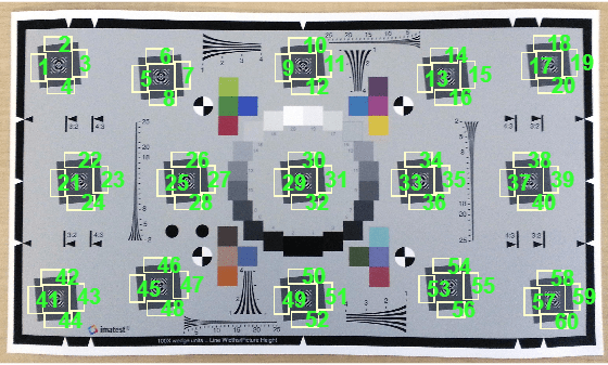
Measure the edge sharpness in ROIs 25-28, and return the measurements in sharpnessTable. Include measurements of the MTF70 and MTF30 by specifying the PercentResponse name-value argument.
sharpnessTable = measureSharpness(chart,ROIIndex=25:28,PercentResponse=[70 30])
sharpnessTable=4×9 table
    ROI    slopeAngle    confidenceFlag        SFR           comment                          MTF70                                           MTF70P                                        MTF30                                       MTF30P
    ___    __________    ______________    ____________    ____________    ____________________________________________    ____________________________________________    ________________________________________    ________________________________________

    25       4.2612          true          {84×5 table}    {0×0 double}    0.061813    0.059159    0.052978     0.06016    0.061813    0.059159    0.052978     0.06016    0.10726    0.11137    0.10976    0.11064    0.10726    0.11137    0.10976    0.11064
    26       5.0749          true          {84×5 table}    {0×0 double}     0.18617     0.18573     0.18613     0.18623     0.18617     0.18573     0.18613     0.18623    0.26279    0.26419     0.2628    0.26398    0.26279    0.26419     0.2628    0.26398
    27       4.7436          true          {84×5 table}    {0×0 double}    0.069296    0.069197    0.064096    0.068951    0.069296    0.069197    0.064096    0.068951    0.21611    0.21953    0.21891    0.21977    0.21611    0.21953    0.21891    0.21977
    28       4.7982          true          {84×5 table}    {0×0 double}     0.19005     0.20272     0.19611      0.1999     0.19005     0.20243     0.19595      0.1999    0.26278    0.27244     0.2617     0.2707    0.26278    0.27228    0.26164     0.2707
Select the fourth row in the sharpness table, which corresponds to ROI 28. Display the SFR plot of the ROI.
idx = 4;
plotSFR(sharpnessTable(idx,:))
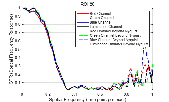
Print the MTF70 and MTF30 measurements of the ROI. Compare the measurements against the plot.
The MTF70 measurement of the red and blue color channels are slightly smaller than 0.2, while the MTF70 measurement of the green and luminance channels are slightly larger than 0.2. These measurements agree with a visual inspection of the SFR plot, on which an SFR value of 0.7 occurs at spatial frequencies around 0.2 line pairs per pixel.
mtf70 = sharpnessTable.MTF70(idx,:)
mtf70 = 1×4

    0.1900    0.2027    0.1961    0.1999
The MTF30 measurement of the blue color channel is noticeably smaller than the MTF30 measurement of the other color channels. This measurement agrees with a visual inspection of the SFR plot, on which the SFR curve of the blue channel drops off more quickly than the other channels.
mtf30 = sharpnessTable.MTF30(idx,:)
mtf30 = 1×4

    0.2628    0.2724    0.2617    0.2707
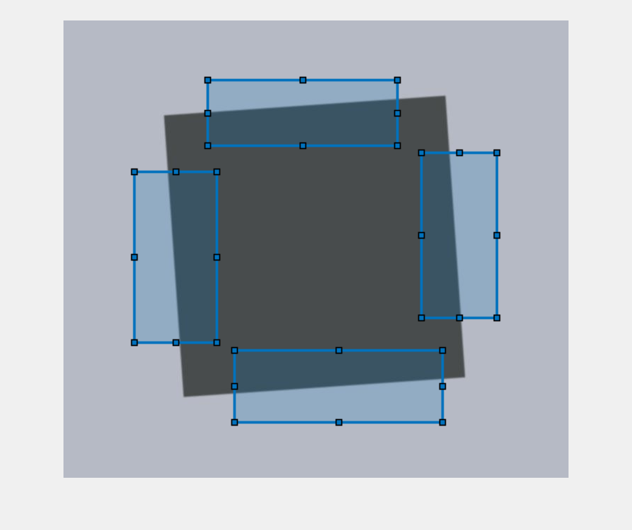
Read and display an image of a custom test chart with slanted edge ROIs.
I = imread("slantedSquare.jpg");
imshow(I)
Draw ROIs for the edges, starting at the top and moving clockwise.
numROIs = 4;
roiPos = zeros(numROIs,4);
for cnt = 1:numROIs
    hrect = drawrectangle;
    roiPos(cnt,:) = hrect.Position;
end
Calculate the SFR, MTF50, and MTF50P for the selected ROIs.
sharpnessValues = measureSharpness(I,roiPos)
sharpnessValues=4×8 table
    ROI    slopeAngle    confidenceFlag         SFR           comment                        MTF50                                       MTF50P                           ROIPosition
    ___    __________    ______________    _____________    ____________    ________________________________________    ________________________________________    ________________________

     1       3.9977          true          { 95×5 table}    {0×0 double}    0.18531    0.18554    0.17757    0.18482    0.18531    0.18554    0.17757    0.18482    205     85    269     93
     2       4.0233          true          {109×5 table}    {0×0 double}    0.18567    0.18623     0.1767    0.18533    0.18567    0.18623     0.1767    0.18533    508    188    107    234
     3       3.9977          true          {104×5 table}    {0×0 double}    0.18401    0.18393    0.17425    0.18317    0.18401    0.18393    0.17425    0.18317    243    468    295    102
     4       3.9827          true          {119×5 table}    {0×0 double}    0.18556    0.18624    0.17595    0.18534    0.18556    0.18624    0.17595    0.18534    101    215    117    242
Input Arguments
Name-Value Arguments
Output Arguments
More About
Tips
Slanted edges on a properly oriented chart are at an angle of 5 degrees from the horizontal or vertical. Sharpness measurements are not accurate when the edge orientation deviates significantly from 5 degrees.
Sharpness is higher toward the center of the imaged region and decreases toward the periphery. Horizontal sharpness is usually higher than vertical sharpness.
Algorithms
The SFR measurement algorithm is based on work by Peter Burns [2]
[3]. First,
measureSharpness determines the edge position with sub-pixel
resolution for each scan line, or row or column of pixels
perpendicular to the edge, in the ROI. For example, each row of pixels is a scan line
for a near-vertical edge. Next, measureSharpness aligns and
averages the scan lines to create an oversampled edge intensity profile. The function
takes the derivative of the intensity profile and applies a windowing function. The
returned SFR measurement is the absolute value of the Fourier transform of the windowed
derivative.
References
[1] Imatest. "Esfr". https://www.imatest.com/mathworks/esfr/.
[2] Burns, Peter. "Slanted-Edge MTF for Digital Camera and Scanner Analysis." Society for Imaging Science and Technology; Proceedings of the Image Processing, Image Quality, Image Capture Systems Conference. Portland, Oregon, March 2000, pp. 135–138.
[3] Burns, Peter. "sfrmat3: SFR evaluation for digital cameras and scanners." URL: http://losburns.com/imaging/software/SFRedge/sfrmat3_post/index.html.